Programming in R

The big picture

In sport and health research you end up with lots of numbers: the heights of a squad, their body mass, their VO₂max (the maximal oxygen uptake from a lab test). R is a free programming language built for exactly this. A programming language is simply a strict way of writing instructions that a computer can follow. Instead of clicking through a spreadsheet, you write the steps down once, and R can redo them for any new data.

The lecture builds R up in layers, like learning a spoken language:

1. Words. You store a value under a name, such as mass <- 70. A named value is called an object.
2. Kinds of words. Every value has a type: a number, a whole number, text, or TRUE/FALSE.
3. Containers. Values travel in containers: a row of values (a vector), a grid (a matrix), a table (a data frame) or a mixed bag (a list).
4. Pointing. Square brackets pick out the part you need, such as "the third athlete" or "everyone taller than 180 cm".
5. Verbs. Functions are ready-made tools, like mean() for an average. You can also write your own.
6. Grammar. if/else chooses between actions; a for loop repeats an action for every athlete.
7. Extra vocabulary. Packages are free add-on toolboxes, for example one for dates.

In class, groups did ten short exercises with their own data: their heights, birthplaces, body mass and VO₂max. This page walks through all ten. The lecture also opened with a poll by Sport Data Valley among "embedded scientists" (data specialists who work inside sports federations and help coaches). Asked which language they would rather learn more about, 50% chose R, 32% Python and 18% had no preference.

Analogy: think of R as a kitchen. Objects are labelled jars, functions are appliances (a blender takes ingredients in and gives a result back), and a script is the written recipe that lets anyone cook the same dish again.

Key terms

Terms are listed in the order you need them; each one only uses terms above it.

• R. A free programming language for working with data. Typing 2 + 3 makes R print 5.
• Console. The window where you type one command and R answers straight away, like a calculator.
• Script. A text file of saved commands (ending in .R) that you can run again later. Example: vo2_analysis.R.
• Comment. Text after a # sign. R ignores it; it is a note for humans. Example: # author: Tomer.
• RStudio. A program wrapped around R (an "integrated development environment") with panes for your script, the console, your stored values, plots and help pages.
• Object. A value stored under a name. Example: the name mass holding the number 70.
• Assignment. Storing a value under a name with the arrow <-. Example: mass <- 70.
• Session. Everything from starting R until you close it. Objects live in the session and disappear when it ends, unless you save them.
• Environment (workspace). The collection of objects that exist in your session right now. ls() lists their names.
• Function. A named tool that takes inputs and gives back a result. You call it with round brackets. Example: sqrt(16) gives 4.
• Argument. An input you hand to a function inside its brackets, sometimes with a name. In round(3.146, digits = 2) the arguments are 3.146 and digits = 2.
• Default. The value an argument takes when you do not supply one. Example: round(3.146) uses digits = 0 and gives 3.
• Return value. What a function hands back. sqrt(16) returns 4.
• Data type. The kind of value. Example: typeof("Delft") says "character" (text).
• Numeric (double). An ordinary number; decimals allowed. Example: 70.5. R calls its storage "double".
• Integer. A whole number stored in a compact way, written with an L. Example: 5L.
• Character (string). Text between quotes. Example: "Maastricht".
• Logical. One of the two answers to a yes/no question: TRUE or FALSE. Example: 3 > 2 gives TRUE.
• Complex, raw, date-time. Rare types: a number with an imaginary part (3+2i), raw computer bytes (charToRaw("hallo")), and dates or times (as.Date("2026-10-20")).
• Class. A label that tells R what kind of object something is and how to print it. It can say more than the type: a date is stored as a double but has class "Date".
• NA. "Not available": the marker for a missing value. Example: a VO₂max test that was never done.
• NULL. "Nothing at all": an empty object. Not the same as a missing measurement.
• Data structure (container). How several values are stored together, and in what shape: vector, matrix, data frame, list.
• Vector. A row of values that all have the same type, made with c() ("combine"). Example: c(176, 183, 192, 177).
• Element. One value inside a container. In c(176, 183), 183 is the second element.
• Index (position). The number of an element's place, counting from 1. In c(176, 183), 183 has index 2.
• Coercion. R quietly converting values to one shared type. Example: c(1, "a") turns the 1 into the text "1".
• Vectorised. An operation that works on every element at once. Example: c(1, 2, 3) * 2 gives 2 4 6.
• Named vector. A vector whose elements carry labels. Example: VO₂max values labelled subject1 to subject4.
• Factor. A vector of categories with a fixed set of allowed values. Example: factor(c("m", "f", "f", "m")).
• Level. One allowed category of a factor. Above, the levels are "f" and "m".
• Matrix. A grid of rows and columns where every cell has the same type. Example: a 2 × 2 grid of heights.
• Array. Like a matrix, but with more than two dimensions, for example person × test × day.
• Data frame. A table. Each column is a vector, all columns have the same length, and different columns may have different types. Example: a height column (numbers) next to a birthplace column (text).
• Observation and variable. In a data frame, a row is one observation (for example one athlete) and a column is one variable (for example height).
• List. A container that can hold anything: different types and different sizes side by side. Example: a name, a number and a vector together.
• Subsetting (indexing). Taking out part of an object, usually with square brackets. Example: height[2].
• Comparison operator. A symbol that asks a yes/no question about values: <, >, <=, >=, == (equal to), != (not equal to). Example: 186 >= 175 gives TRUE.
• Logical operator. Combines TRUE/FALSE answers: & (and), | (or), ! (not). Example: TRUE & FALSE gives FALSE.
• Condition. Any expression whose answer is TRUE or FALSE, used to choose an action or to filter data. Example: height > 180.
• na.rm. An argument of summary functions such as mean(). na.rm = TRUE means "remove missing values first, then calculate".
• if / else. Code that runs one block only when a condition is TRUE, and another block (the else part) when it is FALSE. Each possible path is called a branch.
• Loop, for loop, iteration. A loop repeats code. A for loop runs its code once for each element of a vector; each run is one iteration.
• Package (library). An add-on bundle of functions written by other people. Example: lubridate for dates.
• CRAN. The Comprehensive R Archive Network: the official free online collection of R packages.
• str(). A function that shows an object's structure: its size, its columns and their types.

1. Where you type R: console, script and RStudio

Plain definition. R itself is the engine that does the calculations. You can talk to it in the console: type a command, press Enter, get an answer. A script is a file where you write the commands down first and run them from there. RStudio is the program most people use around R. It has four panes: the script top left, the console bottom left, the environment (your stored objects) top right, and files, plots and help bottom right.

From the lecture: in RStudio, Cmd + Enter on a Mac (Ctrl + Enter on Windows) runs the current script line in the console (04:15).

Why it matters. Typing in the console is fine for a quick sum, but nothing is saved. A script means you (or a teammate, or a reviewer) can rerun the whole analysis later and get the same result. This is called reproducibility.

From the lecture: start every script with a header (goal, date, author, version) and comment your code, or you will not recognise it a year later, like old first-year MATLAB code (03:24). For bigger work use an RStudio project (File → New Project), which reopens your scripts and loaded objects as you left them, and note your R version, because packages can break between versions (09:06).

Worked example: a script header in that style, plus the command that prints your R version. (The lecturer's laptop showed R 4.2.2; the version used for this page is 4.6.1.)

# Goal:    describe the heights of our group (Lecture 2 exercises)
# Date:    2026-10-11
# Author:  Tomer
# Version: 1
R.version.string
#> [1] "R version 4.6.1 (2026-06-24)"

Analogy: the console is a pocket calculator; the script is the recipe card. A calculator answer is gone once you clear it, but a recipe can be followed again tomorrow.

Common confusion. R and RStudio are not the same thing. R does the work; RStudio is the window around it. You can run R without RStudio (the plain "R console" looks like a terminal), but not RStudio without R.

Exam angle. Know why scripts, comments, projects and noting the R version make work reproducible.

In short: R calculates, RStudio is the workspace around it, and a commented script (with a header and the R version) makes your analysis repeatable.

2. Objects and assignment

Plain definition. An object is a value with a name. You create one with the assignment arrow <-, typed as a less-than sign and a minus sign. Read mass <- 70 as "mass gets 70". R first works out the right-hand side, then stores the result under the name on the left. Using the name later gives you the value back.

Why it matters. Every analysis is a chain of named steps. If you can read <-, you can follow any script line by line.

Worked example: this is the lecture's own example. a gets 5. Then b gets a * 2, which is 5 × 2 = 10. Then c gets b^3 (^ means "to the power of"), which is 10 × 10 × 10 = 1000. Typing the name c on its own line prints its value.

a <- 5
b <- a * 2
c <- b^3
c
#> [1] 1000

The [1] in front of the output is not part of the answer. It tells you that the first value on that output line is element number 1. It helps when a long vector wraps over several lines.

Three ways to assign, one recommended.

• some_text <- "Lorem ipsum dolor sit amet" is the recommended way.
• some_text = "Lorem ipsum dolor sit amet" also works, but the slides call it discouraged.
• "Lorem ipsum dolor sit amet" -> some_text (rightward assignment) also works, but the slide says "Don't do this".

From the lecture: = is discouraged because it already sets arguments inside function brackets, as in mean(x, na.rm = TRUE); -> because readers expect the object's name on the left (13:20).

Naming rules. These are the lecture's rules, with the examples from the slide:

• Names cannot start with a number.
• Names cannot contain some special symbols (such as $, ^, !) or spaces.
• Underscores and dots are allowed.
• R is case-sensitive: data and Data are two different objects.

From the lecture: use underscores (or dots) and names that say what the object holds, like body_mass, rather than a, b and c (14:39).

1trial <- 5
#> Error: unexpected symbol in "1trial"

data <- 1
Data <- 2
data
#> [1] 1
Data
#> [1] 2

Listing your objects. ls() lists the names of all objects in your environment. This is the slide's example ('hallo' is Dutch for "hello"):

a <- 0
b <- 'hallo'
my_number <- 1223
ls()
#> [1] "a"         "b"         "my_number"

Correction: storing and comparing are different. mass <- 70 stores 70. mass == 70 asks "is mass equal to 70?" and answers TRUE or FALSE. It changes nothing.

mass <- 70
mass * 2
#> [1] 140
mass == 70
#> [1] TRUE

Analogy: an object is a labelled jar. <- puts something in the jar. Assigning again to the same name empties the jar and puts in the new value.

Predict the output. What does the last line print?

x <- 4
y <- x + 1
x <- 10
y

x <- 4
y <- x + 1
x <- 10
y
#> [1] 5

Exam angle. Expect to trace short assignment chains like the a, b, c example, and to spot names that cause errors.

In short: name <- value stores a value; names are case-sensitive, cannot start with a digit, and should say what they hold; == compares, <- assigns.

3. Data types

Plain definition. Every single value in R has a type: the kind of thing it is. The type decides what you can do with it. You can average numbers, but not words.

typeof(x) tells you how R stores x. The lecture's examples: a holding 0 is a double, b holding 'hallo' is a character, and 5L is an integer.

typeof(a)
#> [1] "double"
typeof(b)
#> [1] "character"
typeof(5L)
#> [1] "integer"
typeof(3.14)
#> [1] "double"
typeof(TRUE)
#> [1] "logical"
typeof(13 + 37i)
#> [1] "complex"
charToRaw("hallo")
#> [1] 68 61 6c 6c 6f
typeof(as.Date("2022-02-02"))
#> [1] "double"
class(as.Date("2022-02-02"))
#> [1] "Date"

What each type is for.

• Numeric is the default for any number you type, with or without decimals.
• Integer stores whole numbers. The L after the number marks it.
• Character is text. Quotes matter: "70" is text, 70 is a number.
• Logical is TRUE or FALSE. R also accepts the short forms T and F. The slide lists NA as a possible logical value too; NA gets its own section below.
• Complex numbers (with an imaginary part, i) are not used in this course.
• Raw stores data as bytes, the basic units a computer stores. charToRaw("hallo") shows the letters h, a, l, l, o as the byte codes 68 61 6c 6c 6f.
• Date-time values hold dates and times, such as 02-02-2022 10:00:00 CET on the slide. They are usually made by converting text.

From the lecture: integers take less memory than numeric values, so calculations on large datasets run faster (10:59). Single and double quotes are equivalent; pick one and be consistent (11:54).

From the lecture: the types you will meet most are numeric, integer, character and logical; for date-times, look at the lubridate package (12:35).

class(x) describes what kind of object something is, which can say more than the storage type. A date is stored as a number (typeof says double: the number of days since 1 January 1970), but its class is "Date", so R prints it as a date.

Correction: a whole number is not automatically an integer. 5 is numeric (double). Only 5L is an integer. The recording is a bit muddled here; the slide's table is right: r <- 5 is "numeric (real)", i <- 5L is "integer".

Exam note: the slide lists "Datetime" next to numeric, integer and so on as a data type. Strictly, a date-time is a class built on top of numbers: typeof() of a date says "double". If an exam question just follows the slide's list, date-time counts as one of the types shown in the lecture. If it asks what typeof() returns for a date, the answer is double.

Illustration: in an athlete database, body mass is numeric (72.4), the number of matches played could be an integer (23L), the club name is character ("Ajax"), and "injured this season?" is logical (TRUE).

Predict the output. What does each line print?

typeof(7)
typeof(7L)
typeof("7")
typeof(7 > 3)

typeof(7)
#> [1] "double"
typeof(7L)
#> [1] "integer"
typeof("7")
#> [1] "character"
typeof(7 > 3)
#> [1] "logical"

Exam angle. Classify values such as 5, 5L, "5" and TRUE by type.

In short: the main types are numeric (double), integer (5L), character (quoted text) and logical (TRUE/FALSE); typeof() tells you which one you have.

4. Containers at a glance

Plain definition. Types describe single values. Data structures (containers) describe how many values are stored together and in what shape. In short, a data type is the kind of value; a data structure is how you organise and store values.

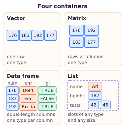
Figure: the four containers you must know. Same colour means same type: vectors and matrices have one type, a data frame has one type per column, and a list can hold anything.

The slides also list NULL under data structures: the empty object (section 12).

Why it matters. Many exam questions are of the type "which container can hold X?". The answer comes from the "Types inside" column.

Exam note: the slide's table describes the factor as "1-dimensional, multiple types", the same as the list. That is loose wording. A factor holds categories from one fixed set of labels (R stores them as whole-number codes plus one label per code; typeof() of a factor says "integer"). It cannot mix numbers and text the way a list can. If an exam question asks which structure can hold several types of values, answer list (and, column by column, the data frame). A past test exam asked exactly this with the options vector, matrix, array and list; the answer was list.

Exam angle. Match a description ("one type per column", "can mix anything") to the right container.

In short: vector = one row, one type; matrix = grid, one type; data frame = table, one type per column; list = anything goes.

5. Vectors

Plain definition. A vector is an ordered row of values of one type. You make one with c(), short for "combine". It is the basic building block of R: even a single number like 5 is a vector of length 1.

Why it matters. A vector is how you hold one measurement for a whole group, for example everyone's height. Most other containers are built from vectors.

Worked example (Exercise 2, parts 1 and 2). In the lecture each group made a vector of their heights in cm and a vector of their birthplaces. These are the values from the lecture's solution:

height <- c(176, 183, 192, 177)
location <- c('Amsterdam', 'De Koog', 'Maastricht', 'Den Haag')
length(height)
#> [1] 4
height / 100
#> [1] 1.76 1.83 1.92 1.77

length() counts the elements: 4. height / 100 converts every height to metres in one go. That is what vectorised means: one instruction, applied to every element.

One type only: coercion. If you mix types in c(), R does not complain. It quietly converts everything to the most flexible type. The order is logical → integer → numeric → character. Text is the most flexible, because anything can be written as text.

c(176, "Delft")
#> [1] "176"   "Delft"
c(1, TRUE, FALSE)
#> [1] 1 1 0

The first line turned 176 into the text "176", so you can no longer calculate with it. In the second line, TRUE became 1 and FALSE became 0.

Handy shortcut. 1:10 makes the whole numbers 1 to 10. sum() of a logical vector counts the TRUEs, because TRUE counts as 1 (DataCamp).

1:10
#>  [1]  1  2  3  4  5  6  7  8  9 10
sum(c(TRUE, FALSE, TRUE))
#> [1] 2

Named vectors (Exercise 3). names() attaches a label to each element. The exercise asked groups to look up what names() does, then label their heights and birthplaces with the group members' names and show them with print(). The slide demonstrates it on VO₂max values in mL/kg/min:

vo2max <- c(54.6, 33.4, 76.1, 23.5)
names(vo2max) <- c('subject1', 'subject2', 'subject3', 'subject4')
print(vo2max)
#> subject1 subject2 subject3 subject4
#>     54.6     33.4     76.1     23.5

The numbers stay the same; each one now has a label above it, so you can see whose value is whose.

Exam note: the slide's title says "Creating a named function using names()". That is a slip: the code makes a named vector (the exercise text itself says "Make a named vector"). names() gives labels to elements; it does not create a function. If asked, call it a named vector.

Predict the output.

c(1, "2", TRUE)
c(2, 4, 6) + 1
sum(c(176, 183, 192, 177) > 180)

c(1, "2", TRUE)
#> [1] "1"    "2"    "TRUE"
c(2, 4, 6) + 1
#> [1] 3 5 7
sum(c(176, 183, 192, 177) > 180)
#> [1] 2

Exam angle. Predict what a mixed c() turns into and what a vectorised operation returns.

In short: c() makes a vector; all elements share one type (mixing forces a conversion, usually to text); operations work on every element at once; names() labels the elements.

6. Factors

Plain definition. A factor is a vector for categories, such as sex, sport or medal. Besides the values, it stores the list of allowed categories, called levels. By default the levels are sorted alphabetically.

Why it matters. Categories behave differently from numbers. A factor tells R "these are groups", which matters later for counting, plotting and models.

Worked example (from the slides):

sex <- factor(c("m", "f", "f", "m"))
sex
#> [1] m f f m
#> Levels: f m
levels(sex)
#> [1] "f" "m"
summary(sex)
#> f m
#> 2 2

R prints the values without quotes and then the levels: f and m (alphabetical). summary() counts how many of each level there are (DataCamp).

From the lecture: levels can be plain groups, like m and f, or have a natural order, like low, medium, high; you set the order with the levels argument and ordered = TRUE (20:58).

Ordered factors. Once the order is set, comparisons such as "higher than low" make sense:

intensity <- factor(c("high", "low", "medium", "low"),
                    levels = c("low", "medium", "high"),
                    ordered = TRUE)
intensity
#> [1] high   low    medium low
#> Levels: low < medium < high
intensity > "low"
#> [1]  TRUE FALSE  TRUE FALSE

Correction: inside, R stores a factor as whole-number codes (1, 2, ...) plus one label per code. Those codes are not measurements. Never average them: the "mean discipline" of road and sprint cyclists means nothing.

discipline <- factor(c("road", "sprint", "road"))
as.integer(discipline)
#> [1] 1 2 1

Analogy: a factor is like a multiple-choice form. The levels are the printed answer boxes; each athlete ticks one. The box number is just a position on the form, not a score.

Predict the output. What are the levels?

levels(factor(c("sprint", "road", "road", "track")))

levels(factor(c("sprint", "road", "road", "track")))
#> [1] "road"   "sprint" "track"

Exam angle. Know that levels are sorted alphabetically by default and that ordered = TRUE adds an order.

In short: a factor stores categories plus their allowed levels (alphabetical unless you say otherwise); ordered = TRUE adds an order; the internal codes are labels, not numbers to calculate with.

7. Matrices and arrays

Plain definition. A matrix is a grid with rows and columns, where every cell has the same type. You make one from a vector with matrix(), saying how many rows (nrow) and/or columns (ncol) you want. An array is the same idea with more than two dimensions.

Why it matters. Matrices are common for purely numerical data, such as test scores of several athletes on several tests. And the way R fills them is a classic trace-the-code question.

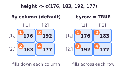
R fills a matrix column by column. Unless you add byrow = TRUE, R puts the first values down the first column, then moves to the next column.

Figure: the same four heights, filled by column (R's default) and by row (byrow = TRUE). The small numbers show the order in which cells are filled.

Worked example (Exercise 2, part 3). Convert the height vector into a 2 × 2 matrix:

matrix(height, nrow = 2)
#>      [,1] [,2]
#> [1,]  176  192
#> [2,]  183  177
matrix(height, nrow = 2, byrow = TRUE)
#>      [,1] [,2]
#> [1,]  176  183
#> [2,]  192  177

In the printout, [1,] means "row 1" and [,2] means "column 2". In the first matrix, row 1 holds 176 and 192, because 176 and 183 filled column 1 first.

The slide's bigger example: the numbers 1 to 10 in 5 rows. R works out that it needs 2 columns, because 10 values / 5 rows = 2.

b <- matrix(1:10, nrow = 5)
b
#>      [,1] [,2]
#> [1,]    1    6
#> [2,]    2    7
#> [3,]    3    8
#> [4,]    4    9
#> [5,]    5   10

From the lecture: write matrix(height, nrow = 2, ncol = 2) rather than matrix(height, 2, 2), so everyone sees which 2 is rows and which is columns; named arguments may come in any order (36:02).

Arrays. An array can have any number of dimensions. With two dimensions it is just a matrix, which is why the slide's array(1:8, c(2, 4)) prints as a 2 × 4 matrix. Illustration: reaction times of 3 athletes × 2 tests × 4 days would fit a 3 × 2 × 4 array.

array(1:8, c(2, 4))
#>      [,1] [,2] [,3] [,4]
#> [1,]    1    3    5    7
#> [2,]    2    4    6    8

One type only. As with vectors, one text value turns the whole matrix into text:

matrix(c(1, 2, "a", 4), nrow = 2)
#>      [,1] [,2]
#> [1,] "1"  "a"
#> [2,] "2"  "4"

Predict the output. Which number ends up in row 1, column 2?

m <- matrix(1:6, nrow = 2)
m[1, 2]

m <- matrix(1:6, nrow = 2)
m
#>      [,1] [,2] [,3]
#> [1,]    1    3    5
#> [2,]    2    4    6
m[1, 2]
#> [1] 3

Exam angle. Trace which value ends up in which cell when a matrix is filled by column.

In short: a matrix is a one-type grid, filled column by column unless byrow = TRUE; name nrow/ncol so it is clear which is which; an array adds more dimensions.

8. Data frames

Plain definition. A data frame is R's table. Each column is a vector, so within a column all values share one type. Different columns can have different types, but all columns must have the same length. Each row is one observation (one athlete); each column is one variable (height, birthplace).

Why it matters. A data frame is a good starting point for storing data and for analysing it column by column.

From the lecture: the data frame is the preferred structure in this course and in the group assignment; the dplyr package (lecture 4) makes processing data frames much easier (19:38).

Look back at the third box in the containers figure (section 4): a set of equal-length columns, each with its own type. The slide shows the same picture, taken from the book Hands-on Programming with R.

Worked example (Exercise 2, part 4). Make a data frame from the height and location vectors. Writing height = height sets the column name (left) and fills it with the vector (right):

group <- data.frame(height = height, location = location)
group
#>   height   location
#> 1    176  Amsterdam
#> 2    183    De Koog
#> 3    192 Maastricht
#> 4    177   Den Haag
str(group)
#> 'data.frame': 4 obs. of  2 variables:
#>  $ height  : num  176 183 192 177
#>  $ location: chr  "Amsterdam" "De Koog" "Maastricht" "Den Haag"

Reading str() output. This is part of data exploration: a first look at what you have.

• 'data.frame': 4 obs. of 2 variables means 4 rows (observations) and 2 columns (variables).
• Each following line is one column: its name after $, its type (num for numbers, chr for text, int for integers, Factor for factors), and its first values.
• With thousands of columns, str() shows only the first ones.

The slide's second example, which section 11 uses again:

d <- data.frame(vo2max = c(22, 33, 44, 55, 66),
                weight = c(70, 72, 74, 76, 78))
d
#>   vo2max weight
#> 1     22     70
#> 2     33     72
#> 3     44     74
#> 4     55     76
#> 5     66     78
str(d)
#> 'data.frame': 5 obs. of  2 variables:
#>  $ vo2max: num  22 33 44 55 66
#>  $ weight: num  70 72 74 76 78

Columns must be equally long. A data frame must stay rectangular:

data.frame(a = 1:3, b = 1:2)
#> Error in data.frame(a = 1:3, b = 1:2) :
#>   arguments imply differing number of rows: 3, 2

From the lecture: columns read from a CSV file (a plain-text spreadsheet file with comma-separated values) sometimes come in as character; convert them, for example with as.numeric(), before calculating (22:34).

vo2_text <- c("54.6", "33.4")
mean(vo2_text)
#> [1] NA
#> Warning message:
#> In mean.default(vo2_text) :
#>   argument is not numeric or logical: returning NA
mean(as.numeric(vo2_text))
#> [1] 44

Exam note: on the slide, the location column of this data frame is printed as <fct> (factor), and the column name is misspelled locatiion. That output comes from R versions before 4.0. Since R 4.0 (2020), text columns stay character (chr) unless you add stringsAsFactors = TRUE, as the run above shows. On the exam, expect text columns to be character in current R.

Analogy: a data frame is a spreadsheet tab with strict rules: one header per column, one kind of entry per column, and no ragged edges.

Predict the output. For the data frame d above, how many observations and variables does str(d) report, and what is nrow(d)?

nrow(d)
#> [1] 5
ncol(d)
#> [1] 2

Exam angle. Read str() output (rows, columns, types) and remember that all columns must have the same length.

In short: a data frame is a table of equal-length columns, each with its own type; str() shows rows ("obs."), columns ("variables") and each column's type; convert text numbers with as.numeric().

9. Lists

Plain definition. A list is an ordered set of slots, and each slot can hold anything: a single number, a word, a whole vector, even a data frame or another list. The slots can differ in type and in size.

Why it matters. Lists are the most flexible container, so they are how R hands back complicated results.

From the lecture: data downloaded from a website or an API (an online data service that programs can query) usually arrive as a list, which you must take apart ("unlist") into a data frame; lists are "very handy but also difficult to decompose" (19:06).

Worked example (from the slides): a list with a text value, two numbers and a vector:

list("a", 1, 4, c(1, 2, 3))
#> [[1]]
#> [1] "a"
#>
#> [[2]]
#> [1] 1
#>
#> [[3]]
#> [1] 4
#>
#> [[4]]
#> [1] 1 2 3

R prints each slot with its position in double brackets, [[1]] to [[4]]. Slot 4 holds a whole vector of three numbers. A vector could never do this, because there every element must be a single value of one shared type.

Illustration: the information about one athlete, with named slots:

athlete <- list(name = "Ari", height = 182, tests = c(42, 45))
str(athlete)
#> List of 3
#>  $ name  : chr "Ari"
#>  $ height: num 182
#>  $ tests : num [1:2] 42 45

unlist() flattens a list into one vector, coercing to one type if needed:

unlist(list(1, 2:3))
#> [1] 1 2 3
unlist(athlete)
#>   name height tests1 tests2
#>  "Ari"  "182"   "42"   "45"

In the second line the numbers became text, because the name "Ari" is text. That is coercion again.

How a data frame relates to a list. A data frame is a special list: each column is one slot, with the extra rule that all slots are vectors of the same length. That rule is what makes it a rectangle.

Exam angle. "Which structure can hold different types and sizes?" The answer is a list.

In short: a list holds anything, of any type and size, in ordered (optionally named) slots; downloaded data often come as lists; unlist() flattens one into a vector.

10. Comparisons and logical values

Plain definition. A comparison operator asks a yes/no question and answers with a logical value, TRUE or FALSE. The six operators from the slide:

Why it matters. Comparisons drive filtering ("only athletes above 180 cm"), if/else decisions and loops.

Worked example (from the slides). 1 is not greater than 2, so FALSE. In 3 >= 2 + 1, R first does the sum (2 + 1 = 3), then asks "is 3 at least 3?": TRUE. Comparing a vector with one number compares every element: 1 > 2 FALSE, 2 > 2 FALSE, 3 > 2 TRUE.

1 > 2
#> [1] FALSE
3 >= 2 + 1
#> [1] TRUE
c(1, 2, 3) > 2
#> [1] FALSE FALSE  TRUE

Combining conditions (DataCamp). & means "and" (both must be TRUE), | means "or" (at least one TRUE), ! means "not" (flips TRUE and FALSE).

h <- c(176, 183, 192, 177)
h > 180 & h < 190
#> [1] FALSE  TRUE FALSE FALSE
h < 177 | h > 190
#> [1]  TRUE FALSE  TRUE FALSE
!(h > 180)
#> [1]  TRUE FALSE FALSE  TRUE

Read the first line per athlete: 176 is not above 180 (FALSE); 183 is above 180 and below 190 (TRUE); 192 is not below 190 (FALSE); 177 is not above 180 (FALSE).

Correction: = and == are different. x = 5 stores 5 in x, like <-. x == 5 only asks whether x equals 5.

Predict the output.

5 != 5
c(60, 75, 90) >= 75
TRUE | FALSE

5 != 5
#> [1] FALSE
c(60, 75, 90) >= 75
#> [1] FALSE  TRUE  TRUE
TRUE | FALSE
#> [1] TRUE

Exam angle. Evaluate a comparison on a vector element by element.

In short: <, >, <=, >=, ==, != return TRUE/FALSE for every element; combine conditions with & (and), | (or) and ! (not); == asks, <- stores.

11. Indexing: picking parts with [ ], [[ ]] and $

Plain definition. Indexing (also called subsetting) means pulling out part of an object. Square brackets after an object's name say which part you want. R counts positions from 1.

From the lecture: Python starts counting at 0, but R starts "where you expect it to start", at 1 (37:17).

Why it matters. Almost every analysis selects something: one athlete, one variable, everyone above a threshold. Tracing what [ ] returns is a classic exam task.

Vectors

The slide's vector a has seven elements: 1, 2, 3, 4, 8, 9, 10. Note that position and value are different things here: position 5 holds the value 8.

Figure: each row is one indexing command; the coloured boxes are the elements it returns.

a <- c(1, 2, 3, 4, 8, 9, 10)
a[2]
#> [1] 2
a[-2]
#> [1]  1  3  4  8  9 10
a[c(1, 2, 7)]
#> [1]  1  2 10
a[3:5]
#> [1] 3 4 8
a[a > 3]
#> [1]  4  8  9 10

• a[2]: the element in position 2.
• a[-2]: a minus sign means "everything except". Position 2 is dropped.
• a[c(1, 2, 7)]: a vector of positions picks several elements at once.
• a[3:5]: positions 3, 4 and 5 (3:5 is short for c(3, 4, 5)).
• a[a > 3]: logical indexing. First a > 3 makes a TRUE/FALSE value for every element: F F F T T T T. Then the brackets keep the elements where it is TRUE. This is how you filter.

Two more things that show up in tracing questions (DataCamp): a position past the end gives NA, and a named vector can be indexed by name.

a[8]
#> [1] NA
vo2max["subject3"]
#> subject3
#>     76.1

Matrices: [row, column]

For anything with rows and columns, the comma separates the two: [row, column]. Leave a side empty to mean "all of them". The slide used the 5 × 2 matrix b from section 7:

b[4, 2]
#> [1] 9
b[2, 2]
#> [1] 7
b[, 2]
#> [1]  6  7  8  9 10
b[1, ]
#> [1] 1 6

b[4, 2] is row 4, column 2: 9. b[2, 2] is 7. b[, 2] has no row number, so it gives all rows of column 2. b[1, ] gives all columns of row 1.

Data frames: [row, column] and $

Data frames take the same [row, column] form, plus the dollar sign. d$vo2max pulls out the whole vo2max column as a vector. These are the slide's examples with d from section 8:

d$vo2max[3]
#> [1] 44
d[2, 1]
#> [1] 33
d[4, 2]
#> [1] 76
d[, 2]
#> [1] 70 72 74 76 78
d[, "weight"]
#> [1] 70 72 74 76 78

• d$vo2max[3]: take the vo2max column, then its third element: 44.
• d[2, 1]: row 2, column 1: 33.
• d[4, 2]: row 4, column 2: 76.
• d[, 2] and d[, "weight"]: all rows of the second column, chosen by position or by name in quotes.

Combine $ and a condition to keep only some rows. Note the comma: the condition picks rows, and the empty spot after the comma keeps all columns.

d[d$vo2max >= 44, ]
#>   vo2max weight
#> 3     44     74
#> 4     55     76
#> 5     66     78

Common confusion: d["weight"] (no comma) returns a one-column data frame, while d$weight and d[, "weight"] return a plain vector.

d["weight"]
#>   weight
#> 1     70
#> 2     72
#> 3     74
#> 4     76
#> 5     78
d$weight
#> [1] 70 72 74 76 78

Lists: [ ] versus [[ ]] versus $

Single brackets on a list return a smaller list. Double brackets [[ ]] or $ take the content out of a slot.

Figure: [ ] gives you a carriage (still a list); [[ ]] and $ give you what is inside it.

athlete["tests"]
#> $tests
#> [1] 42 45
athlete[["tests"]]
#> [1] 42 45
athlete$tests
#> [1] 42 45
athlete$tests[2]
#> [1] 45

athlete["tests"] printed $tests above the values: it is still a list with one slot. athlete[["tests"]] is the vector 42 45 itself, so you can calculate with it or index it again, as in athlete$tests[2].

Analogy: a list is a train. [ ] uncouples a carriage and hands you that carriage, still a (shorter) train. [[ ]] opens the carriage and hands you the cargo.

Predict the output. Use the vector a (1, 2, 3, 4, 8, 9, 10) and the data frame d from above.

a[c(2, 4)]
a[-c(1, 2)]
d$weight[d$vo2max > 40]

a[c(2, 4)]
#> [1] 2 4
a[-c(1, 2)]
#> [1]  3  4  8  9 10
d$weight[d$vo2max > 40]
#> [1] 74 76 78

Exam angle. Trace [ ], [row, column], $ and [[ ]] on small objects and give the exact result.

In short: x[i] picks by position (from 1), by name, or by a TRUE/FALSE condition, and -i drops; tables use [row, column] with an empty side meaning "all"; $ takes a column or list slot; on lists [ ] keeps a list and [[ ]] takes out the content.

12. Missing values: NA, na.rm and NULL

Plain definition. NA ("not available") marks a value that should exist but is unknown, like a VO₂max test an athlete missed. It is not zero, not the text "NA" and not FALSE. NA can appear in a vector of any type.

Why it matters. Real data almost always have gaps. If you do not deal with them, one gap can turn a whole summary into NA.

Worked example (Exercise 5). Exercise 5 asked groups to add one missing value to their VO₂max, height and weight vectors, then adjust the code so they get the same results as before. The VO₂max vector is the one from the slide on missing values. The exercise slide's code is cut off at the right edge; the height and weight vectors below are the lecture's values with one NA added, and they give exactly the slide's outputs 46.9, 728 and 73:

vo2max <- c(54.6, 33.4, NA, 76.1, 23.5)
height <- c(176, 183, NA, 192, 177)
weight <- c(70, 72, 74, 76, NA)
mean(vo2max)
#> [1] NA
mean(vo2max, na.rm = TRUE)
#> [1] 46.9
sum(height, na.rm = TRUE)
#> [1] 728
median(weight, na.rm = TRUE)
#> [1] 73

Without help, mean(vo2max) is NA. R reasons: "one value is unknown, so the average is unknown too". Adding na.rm = TRUE (NA remove) tells R to drop the missing values first. The mean is the sum of the values divided by how many there are:

In words: add up all $n$ observed values and divide by $n$, the number of values you added.

With na.rm = TRUE, $n$ is the number of values that are not missing. Here: (54.6 + 33.4 + 76.1 + 23.5) / 4 = 187.6 / 4 = 46.9 mL/kg/min. The sum of the four known heights is 176 + 183 + 192 + 177 = 728 cm. The median of the four known weights (70, 72, 74, 76) is the middle of 72 and 74, which is 73 kg.

The help page of mean (open it with ?mean; the slide shows it) lists mean(x, trim = 0, na.rm = FALSE, ...). So na.rm is FALSE by default. It is described as "a logical value indicating whether NA values should be stripped before the computation proceeds".

From the lecture: when a summary returns NA, check the help page for an na.rm argument (68:59); writing na.rm = T also works, because R reads T as TRUE (70:22).

Correction: na.rm = TRUE does not fill in or recover the missing value. It just leaves it out. If values are missing for a reason (for example, the least fit athletes skipped the VO₂max test), the average of the rest can be biased.

Finding and counting NAs (DataCamp). is.na() asks "is this missing?" for every element, so sum(is.na(x)) counts the gaps:

is.na(vo2max)
#> [1] FALSE FALSE  TRUE FALSE FALSE
sum(is.na(vo2max))
#> [1] 1

Correction: a comparison with NA gives NA, not FALSE. So filtering with a condition can let an NA slip through:

vo2max > 50
#> [1]  TRUE FALSE    NA  TRUE FALSE
vo2max[vo2max > 50]
#> [1] 54.6   NA 76.1
vo2max[!is.na(vo2max) & vo2max > 50]
#> [1] 54.6 76.1

The middle line returns NA as a third "result": R does not know whether the missing value is above 50. Adding !is.na(vo2max) & keeps only values that are known and above 50.

NULL is different from NA. NA is a placeholder for a value that exists but is unknown; it takes up a slot. NULL is the absence of anything; it takes up no slot:

length(c(1, NA, 3))
#> [1] 3
length(c(1, NULL, 3))
#> [1] 2

Analogy: NA is an empty seat with a name card on it (someone should be there). NULL is no seat at all.

Predict the output.

vo2 <- c(42.1, 51.6, 47.3, NA)
mean(vo2)
mean(vo2, na.rm = TRUE)
length(vo2)

vo2 <- c(42.1, 51.6, 47.3, NA)
mean(vo2)
#> [1] NA
mean(vo2, na.rm = TRUE)
#> [1] 47
length(vo2)
#> [1] 4

Exam angle. Predict mean() with and without na.rm = TRUE, and explain what dropping NAs does and does not do.

In short: NA marks an unknown value and spreads through calculations; na.rm = TRUE drops NAs from a summary but does not recover them; is.na() finds them; NULL means "nothing", not "missing".

13. Using functions and their arguments

Plain definition. A function call has the form function_name(arguments). As the slide puts it: "Just write the name of the function and then the data you want the function to operate on in parentheses". R comes with many functions built in.

Why it matters. Almost everything in R is a function call: c(), mean(), data.frame(), even typeof().

Getting help. ?mean or help("mean") opens the help page. The slide's example, ?typeof, says: "typeof determines the (R internal) type or storage mode of any object".

From the lecture: the help page explains what the function does, which arguments it has and how to set them, with examples at the bottom (40:11).

Arguments by position or by name. You can give arguments in the order the help page lists them, or by name. Named arguments may come in any order:

round(3.1415)
#> [1] 3
round(3.1415, digits = 2)
#> [1] 3.14
round(digits = 2, x = 3.1415)
#> [1] 3.14

The first call uses the default, digits = 0, so 3.1415 becomes 3.

Worked example (Exercise 4). Exercise 4 added a weight vector and a VO₂max vector (in mL/kg/min) next to height and location, and asked for four summaries. These are the slide's values, without missing values:

vo2max <- c(54.6, 33.4, 76.1, 23.5)
height <- c(176, 183, 192, 177)
weight <- c(70, 72, 74, 76, 78)
mean(vo2max)
#> [1] 46.9
sum(height)
#> [1] 728
median(weight)
#> [1] 74
round(vo2max, digits = 2)
#> [1] 54.6 33.4 76.1 23.5

• Mean VO₂max: (54.6 + 33.4 + 76.1 + 23.5) / 4 = 46.9 mL/kg/min.
• Sum of heights: 176 + 183 + 192 + 177 = 728 cm.
• Median weight: the middle of the sorted values 70, 72, 74, 76, 78 is 74 kg.
• Rounding to 2 decimals changes nothing here, because the values have only one decimal.

Rounding, floor and ceiling. round() goes to the nearest value. floor() always goes down to a whole number, ceiling() always up. These are the slide's outputs on the named VO₂max vector:

names(vo2max) <- c('subject1', 'subject2', 'subject3', 'subject4')
floor(vo2max)
#> subject1 subject2 subject3 subject4
#>       54       33       76       23
ceiling(vo2max)
#> subject1 subject2 subject3 subject4
#>       55       34       77       24

Watch negative numbers: floor still goes down, so −3.2 becomes −4.

round(3.146, 2)
#> [1] 3.15
floor(3.8)
#> [1] 3
ceiling(3.2)
#> [1] 4
round(47 / 10) * 10
#> [1] 50
floor(-3.2)
#> [1] -4
ceiling(-3.2)
#> [1] -3

Worked example (Exercise 6). "You want a macro overview of the VO₂max of your group: round VO₂max to the nearest 10th value." Here "nearest 10th value" means the nearest multiple of ten (50, 60, ...), not one decimal place. The slide notes there are multiple solutions and shows two. Both use the VO₂max vector with the missing value:

vo2max <- c(54.6, 33.4, NA, 76.1, 23.5)
round(vo2max / 10) * 10
#> [1] 50 30 NA 80 20
round(vo2max, -1)
#> [1] 50 30 NA 80 20

Solution 1, for 54.6: 54.6 / 10 = 5.46; rounded that is 5; 5 × 10 = 50. Solution 2: digits = -1 means "round to one place left of the decimal point", which is the tens. The NA stays NA either way.

Correction: R does not always round a 5 upward. For a value exactly halfway, R rounds to the even neighbour ("round half to even"), so 0.5 becomes 0 and 2.5 becomes 2:

round(c(0.5, 1.5, 2.5))
#> [1] 0 2 2

Predict the output.

sum(c(168, 182, 175, 190))
median(c(62, 75, 68, 80))
round(c(42.123, 51.678), digits = 2)

sum(c(168, 182, 175, 190))
#> [1] 715
median(c(62, 75, 68, 80))
#> [1] 71.5
round(c(42.123, 51.678), digits = 2)
#> [1] 42.12 51.68

Exam angle. Predict the results of round(), floor() and ceiling(), including negative numbers and rounding to tens.

In short: call a function as name(arguments); ?name shows its arguments and defaults; arguments go by position or by name; round, floor and ceiling round to nearest, down and up, and round(x, -1) rounds to tens.

14. Writing your own function

Plain definition. When you need the same calculation more than once, you can package it as your own function. The slide's template:

function_name <- function(argument_1, argument_2, ...) {
  function body
}

You store the function under a name with <-, exactly like any object. Inside the round brackets you list the inputs (arguments). Everything the function does goes between the curly braces { }, called the body. The function returns the value of the last line of the body. You can also say explicitly what comes out with return(...).

From the lecture: give a function a name that says exactly what it does (71:37).

Why it matters: "Don't repeat yourself". Copying the same lines for every athlete is slow and invites typos. One function, used many times, is shorter and safer.

Worked example (the slide's "Don't repeat yourself"). Two subjects each did three power measurements. We want their average power per kg of body mass. sprintf() puts a number into a sentence; %f is the spot where the number goes, printed with six decimals. Without a function, the calculation is typed out twice:

subject_1_power <- c(100, 11, 120)
subject_1_mass <- 81
sprintf("average power per kg = %f", mean(subject_1_power) / subject_1_mass)
#> [1] "average power per kg = 0.950617"

subject_2_power <- c(145, 150, 145)
subject_2_mass <- 77
sprintf("average power per kg = %f", mean(subject_2_power) / subject_2_mass)
#> [1] "average power per kg = 1.904762"

With a function, the calculation is written once and then reused:

print_average_power <- function(power, mass) {
  sprintf("average power per kg = %f", mean(power) / mass)
}
print_average_power(subject_1_power, subject_1_mass)
#> [1] "average power per kg = 0.950617"
print_average_power(subject_2_power, subject_2_mass)
#> [1] "average power per kg = 1.904762"

What the numbers are: subject 1's mean power is (100 + 11 + 120) / 3 = 231 / 3 = 77; divided by 81 kg that is 0.950617. Subject 2: (145 + 150 + 145) / 3 = 146.67; divided by 77 kg that is 1.904762. Same results, half the code.

Worked example (Exercise 7: absolute VO₂max). The exercise: write a function with the input arguments VO₂max and weight that multiplies the two to get the absolute VO₂max. Relative VO₂max is in mL per kg of body mass per minute. Multiplying by body mass in kg gives mL per minute; dividing by 1000 turns mL into litres:

In words: oxygen use per kg times the number of kg gives total oxygen use; divide by 1000 to go from millilitres to litres.

The slide's solution (with the VO₂max vector that contains an NA and the weight vector 70 to 78):

weight <- c(70, 72, 74, 76, 78)
get_abs_vo2max <- function(vo2max, weight) {
  abs_vo2max <- vo2max * weight / 1000
  return(abs_vo2max)
}
get_abs_vo2max(vo2max, weight)
#> [1] 3.8220 2.4048     NA 5.7836 1.8330

For the first athlete: 54.6 mL/kg/min × 70 kg = 3822 mL/min, and 3822 / 1000 = 3.822 L/min. (R prints 3.8220 because it gives every number in the output the same number of decimals.) The function works element by element, so all five athletes are done at once: element 1 of vo2max with element 1 of weight, and so on. The missing VO₂max gives NA.

Common confusion. In the lecture a student asked why vo2max and weight appear twice. Inside function(vo2max, weight) they are just the names of the inputs, placeholders that exist only inside the function. In get_abs_vo2max(vo2max, weight) they are your real data vectors, which happen to have the same names. The call would work just as well with other names, for example get_abs_vo2max(c(50), c(70)).

Worked example: the shorter version from the original notes, without a helper object, with a plain number:

absolute_vo2 <- function(relative_vo2, mass_kg) {
  relative_vo2 * mass_kg / 1000
}
absolute_vo2(50, 70)
#> [1] 3.5

50 mL/kg/min × 70 kg = 3500 mL/min = 3.5 L/min. No return() is needed, because the last line's value is returned.

From the lecture: with several steps in the body, store the result in a helper object and use return() to state exactly what comes out (80:54).

Default values (DataCamp). Give an argument a default with = in the definition; callers may then leave it out:

power_up <- function(x, y = 2) {
  x^y
}
power_up(3)
#> [1] 9
power_up(3, 3)
#> [1] 27

From the lecture: keep functions in their own script and load them with source(), so your main script stays uncluttered (96:50).

Here the file is written from R just for the demonstration; normally you would create it in RStudio:

writeLines("get_abs_vo2max <- function(vo2max, weight) vo2max * weight / 1000",
           "vo2_functions.R")
source("vo2_functions.R")
get_abs_vo2max(60, 80)
#> [1] 4.8

Predict the output.

f <- function(x, y = 10) {
  x + y
}
f(5)
f(5, 1)
f(y = 1, x = 2)

f <- function(x, y = 10) {
  x + y
}
f(5)
#> [1] 15
f(5, 1)
#> [1] 6
f(y = 1, x = 2)
#> [1] 3

Exam angle. Write a short function with two arguments and the right units, or trace what one returns.

In short: name <- function(args) { body } packages a calculation; the last value (or return()) comes out; argument names are placeholders; state the units (VO₂max: mL/kg/min × kg / 1000 = L/min).

15. Choosing with if / else

Plain definition. An if statement runs a block of code only when its condition is TRUE. else if adds another condition to try next, and else catches everything left over. R checks the conditions from top to bottom and runs only the first block whose condition is TRUE; it skips the rest.

if (condition) {
  # runs when condition is TRUE
} else if (other_condition) {
  # runs when the first is FALSE and this one is TRUE
} else {
  # runs when all conditions above are FALSE
}

Why it matters. Data analysis is full of "if this, do that": label athletes, skip bad trials, flag injuries.

Worked example (from the slides). some_value is 2. Is 2 < 3? Yes, so the first block runs and R prints the message. The else if and else are never looked at. (The slide prints Dutch messages; "Kleiner dan 3" means "smaller than 3".)

some_value <- 2
if (some_value < 3) {
  print("smaller than 3")
} else if (some_value < 10) {
  print("smaller than 10")
} else {
  print("10 or more")
}
#> [1] "smaller than 3"

Worked example (Exercise 8). "Individuals are considered very tall if height is 190 cm or more, tall if 175–189 cm, average if 160–174 cm and short if below 160 cm." The slide's solution, for a height of 186 cm:

height <- 186
if (height >= 190) {
  print('very tall')
} else if (height >= 175) {
  print('tall')
} else if (height >= 160) {
  print('average')
} else if (height < 160) {
  print('short')
}
#> [1] "tall"

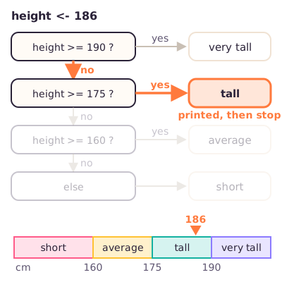
Figure: how R walks down the chain for 186 cm. It stops at the first TRUE, so the later checks never run.

Trace for 186: is 186 ≥ 190? FALSE, so go on. Is 186 ≥ 175? TRUE, so print "tall" and stop.

Order matters. Test the highest threshold first. The second branch only needs height >= 175 (not "between 175 and 189"), because anything 190 or above was already caught by the first branch. The slide's chain ends with else if (height < 160); a plain else would do the same job. These bands are the exercise's labels, not official physiological categories.

From the lecture: usually you write several else ifs and only a plain else at the bottom (85:33).

Illustration: the same checks in the wrong order give the wrong answer, because 186 ≥ 160 is already TRUE:

height <- 186
if (height >= 160) {
  print('average')
} else if (height >= 175) {
  print('tall')
}
#> [1] "average"

The condition must be one TRUE or FALSE. if needs a single, known answer. An NA or a vector of several values gives an error:

if (NA > 5) print("yes")
#> Error in if (NA > 5) print("yes") : missing value where TRUE/FALSE needed

if (c(176, 192) > 180) print("tall")
#> Error in if (c(176, 192) > 180) print("tall") :
#>   the condition has length > 1

From the lecture: put the if/else chain inside a function, so you can label any height in one line (84:55).

height_label <- function(h) {
  if (h >= 190) {
    "very tall"
  } else if (h >= 175) {
    "tall"
  } else if (h >= 160) {
    "average"
  } else {
    "short"
  }
}
height_label(182)
#> [1] "tall"

Predict the output. What does height_label() return for these three heights?

height_label(175)
height_label(189.5)
height_label(159)

height_label(175)
#> [1] "tall"
height_label(189.5)
#> [1] "tall"
height_label(159)
#> [1] "short"

Exam angle. Trace which branch runs for a given value, especially at a boundary such as exactly 175.

In short: if/else if/else runs only the first branch whose condition is TRUE, so put the strictest test first; the condition must be a single TRUE or FALSE (not NA, not a vector).

16. Repeating with for loops

Plain definition. A for loop repeats a block of code once for every element of a vector. The slide's syntax:

for (val in sequence) {
  statement
}

sequence is a vector, and val takes each of its values in turn. In each iteration the statement in the body runs with that value. When the last element has been used, the loop ends. That is the slide's flowchart: "for each item in sequence → last item reached? → no: run the body and go back; yes: exit the loop".

Why it matters. Loops let you apply the same step to every athlete, file or trial. Even when you can avoid them, you must be able to trace one.

Worked example (from the slides). i takes the values 1, 2, 3, 4, 5. Each time, R prints i * 2:

for (i in 1:5) {
  print(i * 2)
}
#> [1] 2
#> [1] 4
#> [1] 6
#> [1] 8
#> [1] 10

From the lecture: the name i is only a convention; you can call the loop variable anything, such as v or n (86:22).

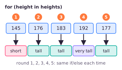
Worked example (Exercise 9). "Use the conditional statement from the previous exercise to get the description of the height of everyone in your group: create a for loop that runs the if-else statement for every group member." The slide's solution puts the whole if/else chain inside the loop body:

heights <- c(145, 176, 183, 192, 177)
for (height in heights) {
  if (height >= 190) {
    print('very tall')
  } else if (height >= 175) {
    print('tall')
  } else if (height >= 160) {
    print('average')
  } else if (height < 160) {
    print('short')
  }
}
#> [1] "short"
#> [1] "tall"
#> [1] "tall"
#> [1] "very tall"
#> [1] "tall"

Figure: in round 1 height is 145, in round 2 it is 176, and so on. The same if/else chain runs each time.

Storing results instead of printing. Printing shows answers but does not keep them. To keep them, make an empty vector first and fill one slot per iteration. seq_along(heights) gives the positions 1, 2, ..., 5:

labels <- character(length(heights))
for (i in seq_along(heights)) {
  labels[i] <- height_label(heights[i])
}
labels
#> [1] "short"     "tall"      "tall"      "very tall"
#> [5] "tall"

While loops (DataCamp). A while loop repeats as long as its condition stays TRUE. Illustration: count 400 m laps until at least 1600 m are run:

distance <- 0
laps <- 0
while (distance < 1600) {
  distance <- distance + 400
  laps <- laps + 1
}
laps
#> [1] 4

Often you need no loop. Because R is vectorised, heights / 100 converts all heights at once. Loops are still worth understanding: follow what changes in each round rather than memorising what the code looks like.

Predict the output.

total <- 0
for (x in c(3, 5, 2)) {
  total <- total + x
}
total

total <- 0
for (x in c(3, 5, 2)) {
  total <- total + x
}
total
#> [1] 10

Exam angle. Trace a loop round by round and give the final value or the printed lines.

In short: for (val in sequence) { ... } runs the body once per element, with val taking each value; store results with an index (labels[i] <- ...); while repeats while a condition holds.

17. Packages: install once, load every session

Plain definition. A package (also called a library) is a bundle of extra functions written by other people. Basic functions like mean() and round() come with R itself, which is why you could use them without installing anything. For anything else there are two steps:

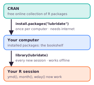
1. install.packages("lubridate") downloads the package from CRAN and installs it on your computer. You do this once per computer. It needs internet, and the package name goes in quotes.
2. library(lubridate) loads the installed package into your current session, so its functions become available. You do this every session (every time you start R). It works offline.

From the lecture: you first need to install a package before you can load it with library(); base functions such as mean() need no installing (98:11).

Figure: installing copies a package onto your computer once; library() loads it into each new session.

Analogy: install.packages() is buying a book and putting it on your shelf. library() is taking it off the shelf and opening it on your desk. You buy it once, but you open it every time you want to read.

Worked example (from the slides). The slide uses lubridate, a package for dates. Before loading it, its functions do not exist:

ymd(20101215)
#> Error in ymd(20101215) : could not find function "ymd"

install.packages("lubridate")
# (once per computer: R downloads the package and prints download messages)

library(lubridate)
#> Attaching package: ‘lubridate’
#>
#> The following objects are masked from ‘package:base’:
#>
#>     date, intersect, setdiff, union
d <- ymd(20101215)
d
#> [1] "2010-12-15"
month(d)
#> [1] 12
wday(d, label = TRUE)
#> [1] Wed
#> 7 Levels: Sun < Mon < Tue < Wed < Thu < ... < Sat

The "Attaching package" message only says that lubridate brings its own versions of a few base functions (they are "masked"); you can ignore it. ymd() reads 20101215 as year-month-day and turns it into the date 2010-12-15. month(d) extracts the month: 12. wday(d, label = TRUE) gives the weekday as a label: Wednesday (Wed). Because weekdays have a natural order, lubridate returns it as an ordered factor, which is why the levels Sun < Mon < ... are printed (section 6).

Which packages? The slide shows a collection of package logos.

From the lecture: the ones singled out were ggplot2 (plots), dplyr (processing data frames) and lubridate (dates); they also appear in the DataCamp modules (99:32).

The others on the slide include tidyr and readr (tidying and reading data), stringr (text), shiny (interactive web apps), rmarkdown and knitr (reports), devtools, packrat, ggvis, and magrittr (which provides the %>% symbol you will meet in lecture 4). You do not need to know every logo; you should know why packages exist. Lecture 4 covers data wrangling (cleaning and reshaping data) and visualisation.

Exercise 10 asked groups to look up which libraries will likely be relevant for the assignments in this course. Tip from the slide: browse the CRAN website.

Correction: the package name needs quotes in install.packages(), because the package is not an object in your session yet. Without quotes, R looks for an object called lubridate and fails:

install.packages(lubridate)
#> Error: object 'lubridate' not found

Exam angle. Know the difference: install once (quotes, internet) versus load every session.

In short: install a package once per computer with install.packages("name") (quotes, internet), then load it every session with library(name); base functions like mean() need no package.