First read: about 5 minutes. Lecture 5: Introduction to machine learning and regression.
Machine learning lets a computer learn a rule (a model) from data. This lecture places it among related fields, then builds a regression workflow (predicting a number, such as jump height) for small sport data sets, where a model can look perfect on measured athletes yet fail on the next one.
The ideas to keep
Blur the explanations and test yourself.
The machine-learning map. Artificial intelligence (AI) contains machine learning (ML), which contains deep learning; data science overlaps with them but is part of neither. Supervised learning uses known answers: regression predicts a number, classification a category. Unsupervised learning finds groups without answers (clustering). Reinforcement learning learns from rewards and penalties.
The regression line and its errors. Prediction = intercept + slope × input: the intercept is the prediction at input 0, the slope the change per unit of input. A residual is actual minus predicted, and least squares picks the line with the smallest sum of squared residuals. MAE averages the residuals' sizes (target's unit); MSE averages their squares (squared unit), so big misses weigh more.
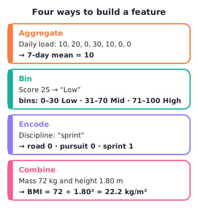
Better inputs. Feature engineering builds better input columns: aggregate (a function of a variable over a window, such as the 75th percentile of jump height over 7 days), bin values into groups, encode categories as 0/1 columns (one-hot: one per category; dummy: one fewer) and combine variables (BMI).
Overfitting and honest testing. A model that fits its training data (the examples it learns from) too closely learns their noise and fails on new athletes, especially in small samples. So lock away about 20% as a test set, used once at the end, compare models with cross-validation (parts of the training data take turns as the scoring set), keep each athlete on one side of every split, and beat a naive baseline with no predictors.
Ridge and LASSO. Both add a penalty for steep slopes to least squares: ridge adds λ × slope², LASSO λ × |slope|, with λ the penalty strength. Ridge shrinks slopes; LASSO can set them to exactly zero, dropping useless inputs. LASSO suits many useless inputs, ridge mostly useful ones.
Deep learning. It finds its own input features, where classical ML needs them built by hand, at the cost of control, interpretability and much more data. For small movement-science data sets, keep it simple.
What to be able to do
Type a scenario's learning task and name its predictors and target.
Compute residuals, MAE and MSE with units.
Name an aggregate's function, variable and window; explain the dummy variable trap.
Spot overfitting; explain the locked test set, k-fold cross-validation, data leakage and the naive baseline.
Redo the λ = 1 ridge and LASSO calculations (1.69 versus 0.74; 0.90).
Answer "which model, and how would you split the data?" for a small athlete data set.
Got the big picture?Mark the overview done to fill this lecture's ring.
2Step 2 of 312–18 min
Detailed notes
This lecture places machine learning among its neighbouring fields, then builds one regression workflow for small sport data sets: fit a line, score its misses, build good inputs, test honestly, and add a penalty (ridge or LASSO) when data are scarce.
Four fields. Artificial intelligence (AI) is the broad field of making machines seem intelligent: able to make the right decision from a set of inputs and possible actions. Machine learning (ML) is the part of AI in which the computer learns its rule, the model, from data instead of being programmed with it. Deep learning is the part of ML that uses neural networks (networks of simple calculating units) with several layers (Section 10). So AI ⊃ ML ⊃ deep learning; AI and ML are not synonyms. Data science, getting knowledge out of data from cleaning to communicating, overlaps with AI and ML but is neither inside nor around them: much of it (data preparation, statistics, visualisation) uses no AI.
Three ways to learn.
Supervised learning. Every training example comes with the answer, and the model learns to predict it. Regression predicts a number (a 10-km time); classification predicts a category (injured or not).
Unsupervised learning. There are no answers; the algorithm finds structure itself. Clustering groups similar cases; dimension reduction squeezes many variables into a few (Lecture 6).
Reinforcement learning. Trial and error: a right decision earns a reward, a wrong one a penalty, and the algorithm improves over many cycles, like a robot finding the exit of a maze.
To type a scenario, look at the target. A coach who predicts finish times in seconds from past athletes' training data has known numbers to learn from, so the task is supervised regression.
Classification vs clustering. Both sort cases into groups. In classification the groups are given beforehand as labels; in clustering the algorithm invents them.
From the lecture: give an algorithm sprinters' and long jumpers' 100-m times with their discipline and it learns to classify, testing whether discipline goes with sprint speed. Give it only the times and ask for two clusters: if both clusters mix the disciplines, something other than discipline may drive sprint speed, a new hypothesis. Supervised learning tends to test hypotheses; unsupervised learning tends to generate them.
Predictors and target. The target (outcome) is what you predict; the predictors (features, inputs) are what you predict it from: predictors → model → target. In "how sprint time is explained by leg power" or "how sprint time depends on leg power", sprint time is the target and leg power the predictor.
The data science lifecycle, nine steps from defining the problem to deployment, is taught in Lecture 1. This lecture works inside two of its steps: feature engineering and data modelling.
2. The regression line, residuals and least squares
A regression line predicts the target from one input:
Here ŷ ("y-hat") is the prediction, β₀ is the intercept, the prediction when the input x is 0, and β₁ is the slope, the change in prediction per one-unit increase in x.
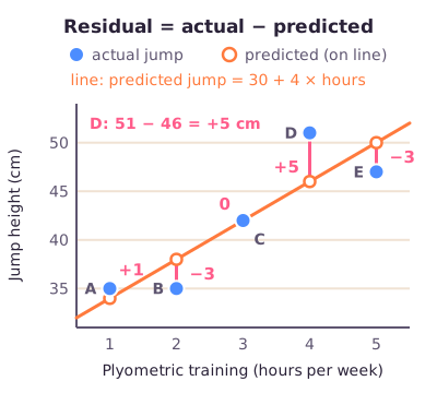
Illustration: five athletes, A to E, do 1 to 5 hours of jump training per week and jump 35, 35, 42, 51 and 47 cm. Their best line is predicted jump = 30 + 4 × hours: 30 cm at 0 hours, plus 4 cm per extra weekly hour.
A residual is actual minus predicted, , measured vertically in the target's unit. The line predicts 34, 38, 42, 46 and 50 cm, so the residuals are +1, −3, 0, +5 and −3 cm. A positive residual means the model guessed too low.
Figure: Each segment is a residual: the vertical gap between a dot (actual) and the line (predicted).
Least squares (ordinary least squares, OLS) chooses the line with the smallest sum of squared residuals (SSR). For the jumpers, SSR = 1 + 9 + 0 + 25 + 9 = 44 cm², and no other straight line gets lower. Least squares only tries to fit the training data (the data the model learns from); it cannot notice when that fit is too good (Section 5).
Line or curve? Long-jump distance rises with run-up speed only up to a point, so a curve (a polynomial, with x², x³… terms) fits better there. But curves are harder to explain, since "more is better" holds only up to the peak, and can be badly wrong for new athletes outside the fitted range.
3. Scoring the misses: MAE and MSE
Averaging the residuals is useless, because positive and negative misses cancel: +1 − 3 + 0 + 5 − 3 = 0. Two loss functions, formulas that turn all residuals into one error number, avoid this:
In words: MAE (mean absolute error) drops each residual's sign and averages over the n cases; MSE (mean squared error) squares each residual and averages.
Worked example: the jumpers' residuals are +1, −3, 0, +5 and −3 cm, so n = 5.
MAE: absolute values 1 + 3 + 0 + 5 + 3 = 12 cm, and 12 ÷ 5 = 2.4 cm. The line misses by 2.4 cm on average.
Athlete D's 5 cm miss is 42% of the MAE sum (5 of 12) but 57% of the MSE sum (25 of 44): squaring gives the largest miss extra weight.
MAE
MSE
Each residual counts
Equally
By its square
Outliers, large errors
Less sensitive
More sensitive, punished more
Direction of the error
Ignored
Ignored
Unit
Target's unit (cm)
Squared unit (cm²)
MSE is not MAE squared (2.4² = 5.76, not 8.8). Because both drop the sign, neither shows whether a model systematically predicts too high or too low; the signed residuals do.
4. Feature engineering: building good inputs
A feature is one input column, and feature engineering means building better features from raw data, because a model can only learn what its features contain. Better features bring flexibility (less complex models that are faster, easier to understand and easier to maintain), simpler models (the features represent the underlying problem better) and better results.
Figure: The four feature operations, each with a before and after.
Aggregate: many values into one
An aggregate feature has three parts: the variable being summarised (jump height), the function that summarises it (mean, median, sum, count, minimum, maximum, percentile, standard deviation, variance) and the window, the stretch of time or data it covers (the previous 7 days, one gait cycle).
Worked example: "top-25% of jump height in the previous 7 days". The top 25% starts at the 75th percentile, the value with 75% of the jumps below it. So the function is the 75th percentile, the variable is jump height and the window is the previous 7 days. In general, "top-X%" means the (100 − X)th percentile.
Illustration: a week of heart-rate recovery values is 32, 30, 34, 31, 8, 33 and 29 beats per minute, and the 8 is a sensor glitch. The 7-day minimum is 8, so one bad reading decides the feature; the 25th percentile is 29.5. A minimum rests on a single value, which could be an outlier, so a percentile is steadier. Percentiles are not always better, though: pick the function that captures what you want to measure.
Bin: values into broader groups
Numerical binning turns numbers into categories: scores 0–30 → Low, 31–70 → Mid, 71–100 → High, or temperatures into low, moderate and high. Categorical binning merges many categories into fewer, such as Spain and Italy → Europe, which helps when each country holds only a few athletes. Binning relabels each value, so it loses the differences inside a bin: 25 and 29 both become "Low". Aggregating, by contrast, summarises many values into one number.
Encode: categories into numbers
Most models only calculate with numbers, so a category column becomes 0/1 indicator columns, where 1 means "belongs to this category". One-hot encoding makes one column per category (k columns for k categories). Dummy encoding leaves one category out (k − 1 columns); that reference category is coded all 0.
Worked example: three cyclists' disciplines, with road as the reference.
Rider
One-hot: road, pursuit, sprint
Dummy: pursuit, sprint
A (road)
1, 0, 0
0, 0
B (pursuit)
0, 1, 0
1, 0
C (sprint)
0, 0, 1
0, 1
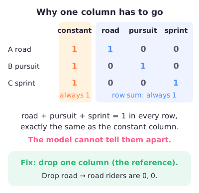
The dummy variable trap. A regression with an intercept acts as if every row had a hidden column of 1s. With all three one-hot columns, road + pursuit + sprint = 1 in every row, which repeats that hidden column, so the model cannot split the effect between them. Dropping the reference column removes the duplicate. The intercept then is the reference category's prediction (road riders), and each dummy's slope is that category's difference from road.
Figure: The one-hot columns always add up to the intercept's constant column.
From the lecture: never code a category as one number column (Italy = 1 … United States = 100). The model reads the codes as amounts, as if the United States were 100 times Italy, and a spurious link with salary can appear.
Combine: a new variable from several
Worked example: BMI = mass ÷ height². For 72 kg and 1.80 m: 1.80² = 3.24, and 72 ÷ 3.24 ≈ 22.2 kg/m². One feature now captures mass relative to height.
5. Overfitting
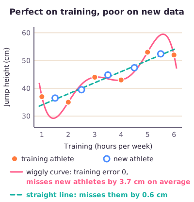
A model generalises when it predicts new cases about as well as its training cases. Overfitting means it fits the training data so closely, random noise included, that it predicts new data badly. Small samples make it much more likely.
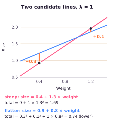
Worked example: the lecture's two-point example. On the full data set, least squares gives size = 0.9 + 0.75 × weight. Keep only two points as training data and treat the rest as test data. Least squares now draws a line straight through the two points, size = 0.4 + 1.3 × weight, with an SSR of 0. It is much steeper, and its squared residuals on the test points are large. Perfect training fit, poor predictions, caused by a tiny sample: overfitting.
Figure: Invented jump data. The curve has zero training error but misses new athletes; the plain line stays close to them.
The sign of overfitting is a large gap: much better scores on training data than on test data. In bias–variance terms (Lecture 6) that gap signals high variance: a model that would change a lot with a different training sample. For the same reason, a high correlation r or R² (the share of the target's variation the model explains) on the whole data set is only half the story: it shows the model fits these data, not that it predicts new ones.
6. Honest testing: holdout, cross-validation and leakage
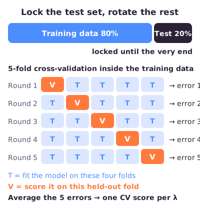
Holdout. Before any modelling, split the data into a training set (about 80%) and a test set (about 20%). Build and tune the model on the training set only. Lock the test set away until the very end, then use it once: predict the test athletes with the final model and compare with their real values, for example as an MAE. Any choice made with the test set, even picking the penalty strength λ (Section 8), makes the reported error too optimistic, because those data are no longer unseen. A small test set, say 9 athletes, also makes the score depend on who landed in it; the strongest check is data from elsewhere, such as another lab (external validation).
The full supervised workflow: data → cleaning → feature engineering → split → train on training data → score test data → evaluate.
Cross-validation assesses how a model's results will generalise to an independent data set, and it suits limited data. k-fold cross-validation works inside the training set only:
Cut the training data into k equal parts, called folds (for example k = 5).
Fit the model on k − 1 folds and score it on the fold left out, the validation fold.
Rotate until every fold has been left out once.
Average the k scores into one cross-validation (CV) score.
Figure: The test set stays locked; each of five training folds takes one turn as the validation fold.
Use CV scores to compare options: least squares versus ridge versus LASSO, or different λ values. Refit the winner on all training data, then unlock the test set once. You never keep the single best fold; the k scores are averaged.
Data leakage is information from the test side seeping into training, which makes results look better than they are.
From the lecture: if an athlete has several rows (sessions, a season), split by athlete: all of that athlete's rows go into training or all into testing, and the same for CV folds. Otherwise the model partly recognises the athlete. With one row per athlete, a random split of rows is fine.
7. The naive baseline
A naive baseline is a model with no predictors, such as "always predict the training-set mean". Compare your model with it on the test set: a model that does not beat it has shown no added predictive value. It is the extreme high-bias (too simple) model; Lecture 6 covers it with the bias–variance trade-off. A low R² can also come from a restricted range, a sample in which a variable hardly varies, rather than from the absence of a relationship; see Lecture 3.
8. Ridge regression
Ridge regression keeps the least-squares score and adds a penalty for steep slopes:
In words: the sum of squared residuals plus λ times the slope squared. Ridge picks the line with the lowest total.
λ (lambda) is the penalty strength, from 0 to infinity. With several predictors the penalty adds all squared slopes, λ × (β₁² + β₂² + …); the intercept is not penalised. The aim is a line that does not fit the training data too well: a larger SSR there in return for a smaller one on test data.
Worked example: the lecture's λ = 1 calculation, on the two training points from Section 5.
Figure: The steep line hits both points; the flatter line misses them but has a much smaller slope.
Steep least-squares line, size = 0.4 + 1.3 × weight. It passes through both points, so SSR = 0. Penalty = λ × slope² = 1 × 1.3² = 1.69. Total = 0 + 1.69 = 1.69.
Flatter line, size = 0.9 + 0.8 × weight. Its residuals are −0.3 and +0.1, so SSR = 0.09 + 0.01 = 0.10. Penalty = 1 × 0.8² = 0.64. Total = 0.10 + 0.64 = 0.74.
The lower total wins: 0.74 < 1.69, so ridge prefers the flatter line even though it fits the training points worse.
Why flatter is safer. With a slope of 1, one extra unit of weight adds one unit of predicted size; with a slope of 2, it adds two. A steep slope makes the prediction very sensitive to small changes in weight; a small slope makes it less sensitive. So ridge predictions are less sensitive to weight than the least-squares line's.
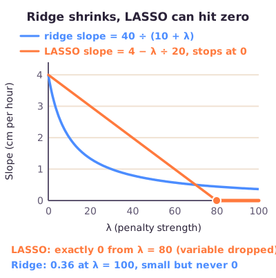
What λ does. λ = 0 means no penalty: plain least squares. As λ grows, the slope gets smaller; with an enormous λ the line goes flat at the mean, which is the naive baseline. Ridge shrinks slopes towards zero but never makes them exactly zero. Choose λ by cross-validation: the λ with the lowest average error on the validation folds, never on the locked test set.
9. LASSO, and choosing a model
LASSO uses the same idea but penalises the slope's absolute value:
Worked example: the same flatter line with λ = 1. SSR = 0.3² + 0.1² = 0.10, as before. Penalty = 1 × |0.8| = 0.8. Total = 0.10 + 0.8 = 0.90. The steep line would score 0 + 1.3 = 1.30, so LASSO also prefers the flatter line.
Why LASSO can remove variables. Near zero, ridge's squared penalty almost vanishes (0.1² = 0.01), so ridge stops pushing the slope down. LASSO keeps charging the same per unit of slope (|0.1| = 0.1). If an input does not earn its cost, the cheapest slope is exactly 0, and the input drops out of the model.
Figure: The invented jumpers from Section 2. The ridge slope shrinks but never reaches 0; the LASSO slope hits exactly 0 at λ = 80, dropping training hours from the model.
Choosing between them. Ridge and LASSO are more robust to overfitting than least squares, especially in small data sets. LASSO beats ridge when many unnecessary features are included, because their slopes turn to zero. Ridge beats LASSO when most features are meaningful. For a numeric target the menu is linear, polynomial, ridge and LASSO regression, plus ensembles such as random forest (Section 10); compare candidates with cross-validation.
Answer pattern: "which model, and how would you split the data?" For a small athlete data set:
Task. Name the target and its type: a number → supervised regression; a category → classification (Lecture 6).
Model. With few athletes for the number of predictors, least squares risks overfitting, so use a penalised regression: LASSO if some predictors are probably useless or you must say which ones matter, ridge if each predictor was picked because it plausibly matters. Skip deep learning: too little data, and it cannot explain its predictions.
Split. Split by athlete: about 80% training and 20% test, the test set locked and used once to estimate performance on new athletes.
Tune. Inside the training set, k-fold cross-validation chooses λ and compares models.
Check. Report the test error next to a naive baseline, and note that a small test set makes the result depend on the split.
Worked example: a coach has 42 handball players, one row each, and 9 candidate predictors of 30-m sprint time (s), such as jump height, leg lean mass and age. She wants to know which predictors matter.
Model: sprint time is a number, so supervised regression. With 42 players and 9 predictors, least squares would likely overfit. Use LASSO: its λ × |slope| penalty shrinks slopes and sets useless predictors to exactly 0, which also shows which ones matter.
Split: about 34 players for training, 8 in a locked test set. Within the 34, 5-fold cross-validation chooses λ and checks LASSO against least squares. Refit on all 34, predict the 8 test players once, and compare the MAE (s) with a baseline that always predicts the training-mean sprint time. Eight players is few, so that MAE is a first estimate.
10. Ensembles, neural networks and deep learning
Ensembles combine several models into one prediction, usually many decision trees, models that predict through a series of yes/no questions. In boosting (AdaBoost, XGBoost) each new tree learns from the errors of the trees before it. In bagging many trees are each trained on a random resample of the data and their predictions are averaged or voted; a random forest is the best-known example. Ensembles do regression and classification; recognising these names is enough.
Neural networks are built from artificial neurons. Each neuron multiplies its inputs by weights (how much each input counts), adds them up, and outputs 1 if the sum passes a threshold: inputs 10, 7 and 3 with weights 0.5, 1.0 and 0.1 give 5 + 7 + 0.3 = 12.3, above a threshold of 10, so the output is 1. Learning means adjusting the weights after wrong predictions.
Deep learning uses neural networks with more than one layer. The key contrast is who builds the features:
Classical ("shallow") ML: input → a human does the feature extraction → model → output.
Deep learning: input → the network extracts the features and predicts → output.
Automatic feature extraction is powerful for complex inputs such as images, but it has three costs. You lose control: domain knowledge is not in the numbers, so a variable you know matters can be weighted near zero. The model is a black box: it is very hard to trace why it predicted what it did. And it needs data: with little data, deep and classical ML perform about the same; as data grow, classical ML levels off while deep learning keeps improving.
From the lecture: movement-science data sets are usually small, so "keep it simple" and use shallow methods. Researchers usually want to know what makes a good sprinter, not only whether someone is one.
Exam traps
A line that fits two training points perfectly and test points badly is overfit to the training data, not "to the testing data".
λ is chosen on the validation folds inside cross-validation. "Lowest residuals for test data" means those folds, never the locked test set.
One-hot = k columns; dummy = k − 1 with the reference coded all 0. The lecturer once swapped the names; answer with these definitions.
"Top-25%" = 75th percentile = the function; jump height = the variable; 7 days = the window.
"Dummy distances" is not an aggregate; mean, median, minimum and percentile are.
Temperatures into low/moderate/high = numerical binning; countries into continents = categorical binning. Neither is clustering.
Cross-validation, the lecturer's top emphasis, assesses how a model generalises to an independent data set. It is not removing outliers, validating raw data or merely splitting the data.
A naive baseline is a model without predictors, not a perfect model and not "using baseline values".
Training error far below test error = overfitting = high variance.
Ridge (slope²) never reaches exactly 0; LASSO (|slope|) can, so it removes variables.
Deep learning extracts features automatically; classical ML needs manual feature engineering.
Worked through the deep dive?Tick it off. Come back to any section whenever you need it.
3Step 3 of 35–8 min
Practice questions
2 exam-style questions. Exam-style open questions: short, with the points shown like on the real exam. Write your answer in the box, then check it against the model answer and the marking guide.
Question 1 — Choose a model and a data split (4 points)
A coach wants to predict how many days athletes need to recover after a hard session. You have one row per athlete for 48 athletes, with 16 measured variables each (for example training load, sleep, heart rate), and some of these variables probably don't help. State and motivate briefly: 1) Which model would you choose and why? (2 points) 2) How would you split your data to check the model, and why? (2 points)
Show answer and rationale
1) A regression model, because the outcome (days of recovery) is a number. With only 48 athletes and 16 variables, several of them probably useless, choose LASSO (ridge is also acceptable): its penalty shrinks the slopes and can set useless variables exactly to zero, which keeps the model from fitting noise (overfitting).
2) Split the athletes into a training set (about 80%) to build the model and a test set (about 20%) that you lock away and use only once at the end, to see how well the model predicts new athletes. Within the training set, use k-fold cross-validation (for example 5 folds: fit on 4, score on the 5th, rotate and average) to choose λ and compare models; with so few athletes this uses the data efficiently and keeps the test set untouched. Also compare with a naive baseline that always predicts the average recovery time.
How the points are earned
1 pt Regression, because the outcome (recovery days) is a number
1 pt LASSO (or ridge), because the sample is small and several variables are useless: the penalty shrinks or removes slopes and limits overfitting
1 pt Training/test split (e.g. 80/20); the test set is used only once at the end to judge predictions for new athletes
1 pt Cross-validation inside the training set to choose λ or compare models
How did your answer compare?
Question 2 — Aggregation versus binning (3 points)
To predict 10-km race time, a coach builds two features from runners' daily training distances: feature A is the top-10% of daily running distance over the previous 14 days, and feature B labels each day's distance as short (< 5 km), medium (5–15 km) or long (> 15 km). State and motivate briefly: 1) Name the aggregate function, the variable and the window of feature A. (1.5 points) 2) How does binning (feature B) differ from aggregation, and what information does it lose? (1.5 points)
Show answer and rationale
1) Function: the 90th percentile (the top 10% starts at the 90th percentile; 90% of the days lie below it). Variable: daily running distance. Window: the previous 14 days.
2) Aggregation summarises many values (here 14 days) into one number, using a function over a window. Binning keeps one value per day but relabels each value into a broader category. It loses the differences within a bin: a 6-km run and a 14-km run both become 'medium'.
How the points are earned
0.5 pt Function: 90th percentile
0.5 pt Variable: daily running distance
0.5 pt Window: the previous 14 days
1 pt Aggregation summarises many values over a window into one number; binning relabels each single value into a category
0.5 pt Binning loses the differences within a bin (e.g. 6 km and 14 km are both 'medium')