Lecture 7 prepares features (the input columns a model uses): putting them on comparable scales and handling empty cells. It ends with neural networks versus simple models, and with risk and odds.
The ideas to keep
Blur the explanations and test yourself.
Scaling changes distances. K-nearest neighbours (KNN) classifies a person by a vote among the closest people in the training data. Age in years differs by tens, height in metres by tenths, so age dominates every distance purely because of its units. In the lecture, scaling alone raised KNN's accuracy from 0.46 to 0.85.
Z-score and min–max. A z-score is (value − mean) ÷ standard deviation (SD), giving mean 0 and SD 1. Min–max is (value − minimum) ÷ (maximum − minimum), giving 0 to 1, and one outlier squeezes the rest. With mean 170 cm, SD 10 cm and range 150–200 cm, 180 cm gives z = 1 and min–max 0.6. Neither changes the shape of the distribution.
Log transformation. A log turns equal ratios into equal steps: with base 2, 1, 2, 4 and 8 become 0, 1, 2 and 3. It changes the shape by pulling very high values in, so it suits features with a few very high values.
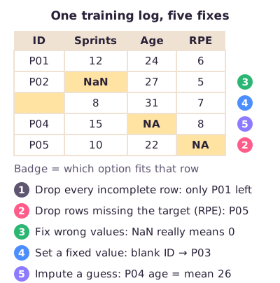
Missing data: five options. Delete incomplete rows; delete only rows missing an essential variable; correct wrong values (a "not a number" cell that is really 0 becomes 0); set a harmless fixed value, such as a missing ID; or impute a best guess, such as the mean. An imputed value is a guess, not a measurement.
Multiple imputation with mice. The R package mice fills each gap several times. With m = 5 you get five completed copies of the data; how much they differ shows how uncertain the guesses are. complete(my_imp, 5) returns copy number 5.
Neural networks. Each node takes a weighted sum of its inputs, subtracts a threshold and applies an on/off rule; layers of nodes fit complex patterns. But networks need much more data and are hard to interpret, and sport and health need explainable predictors, so the course uses simple models.
Risk versus odds. Absolute risk is outcome ÷ everyone in the group (20 of 100 = 0.20); odds are outcome ÷ no outcome (20 ÷ 80 = 0.25). The relative risk (RR) and odds ratio (OR) compare two groups; 1 means no difference. Report a relative risk only with the absolute risk.
What to be able to do
Calculate a z-score and a min–max value; say which transformations keep the shape.
Choose a missing-data option for a given case, including mean replacement and interpolation.
Read a mice() call: m, maxit, the methods and complete().
Calculate absolute risk, odds, RR and OR from a 2×2 table, and say why a study that picks people by outcome gives only an OR.
Got the big picture?Mark the overview done to fill this lecture's ring.
2Step 2 of 312–18 min
Detailed notes
Lecture 7 covers rescaling features (the input columns a model uses), handling missing values, why the course prefers simple models over neural networks, and calculating and reporting risk and odds.
K-nearest neighbours (KNN) classifies a new person by finding the k closest people in the training set (the data the model learns from) and letting them vote. "Closest" is the straight-line distance on a scatter plot of the features:
In words: square the height gap and the age gap, add them, and take the square root.
KNN has no weights of its own, so whatever changes the distances changes its predictions. In any model that relies on distances or variability, the feature with the largest range dominates. In the lecture's data, training heights ran from about 1.50 to 1.96 m and ages from 21 to 38 years. So a 25 cm height gap counts for less than one year of age, though height is what separates men from women.
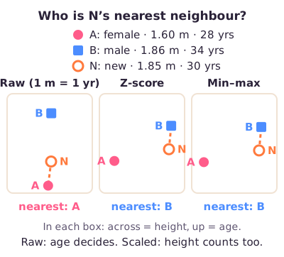
Worked example: three invented students, using the lecture's spreads. Who is nearest to the new student N (1.85 m, 30 years)? A is female (1.60 m, 28 years); B is male (1.86 m, 34 years).
In raw units, N to A is and N to B is . A is nearer, so KNN says "female"; the big height gap adds only 0.0625. Now divide each gap by that feature's standard deviation (SD: 0.13 m for height, 4.85 years for age), which is what z-scoring does. N to A becomes and N to B . B is now nearer, so KNN says "male". Dividing by each feature's range (min–max) gives the same switch: 0.57 versus 0.24.
Figure: In raw units only age matters. After scaling, height counts too.
Only the division rebalances the features. Subtracting the mean or the minimum shifts everyone equally, so no gap changes. That is why centering, subtracting the mean alone, does not make predictors comparable: each gets mean 0, but heights still vary by tenths of a metre and ages by years.
2. Z-score, min–max and log
Z-score (standardization). A z-score says how many SDs a value lies from the mean:
In words: subtract the mean , then divide by the SD . The feature ends up with mean 0 and SD 1. In R: scale(). This is the course's answer to "how do you make all predictors weigh equally?"
Min–max (normalization). Min–max scaling gives a value's position between the smallest and the largest value:
In words: how far above the minimum, divided by the full range. The minimum becomes 0, the maximum 1.
Worked example: a training set has mean 170 cm, SD 10 cm, minimum 150 cm and maximum 200 cm. A player of 180 cm gets z = (180 − 170) ÷ 10 = 1, one SD above the mean, and min–max (180 − 150) ÷ (200 − 150) = 30 ÷ 50 = 0.6, 60% of the way from shortest to tallest. A player of 165 cm gets z = −0.5 (below the mean, so negative) and min–max 15 ÷ 50 = 0.3.
Two consequences for min–max. One extreme value sets the maximum, becomes 1 and squeezes everyone else towards 0; z-scores have no fixed range, so an outlier just gets a large z. And a new value outside the training range falls outside 0–1: with a training minimum of 10 and maximum of 30, a new 40 becomes (40 − 10) ÷ 20 = 1.5, meaning "beyond the training range".
Both methods only shift and stretch the values, so the histogram keeps exactly its shape. A skewed feature stays skewed; z-scoring does not make data normal.
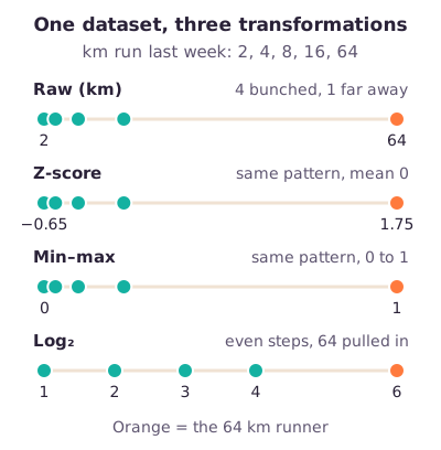
Log transformation. The base-2 logarithm of a number is the power of 2 that gives it: because . So 1, 2, 4 and 8 become 0, 1, 2 and 3. A log turns ratios into differences:
In words: the step between two values depends only on their ratio, so every doubling (2-fold change) is one equal step. That is why fold changes are plotted on log axes.
Unlike the other two, a log changes the shape: large values are pulled in towards the rest. That makes it the tool for right-skewed features (most values low, a few very high). It tames the outliers and often makes the data more symmetric, but does not guarantee normality. A log has no fixed range and works only for positive values (log 0 is undefined).
Figure:Illustration. Five people ran 2, 4, 8, 16 and 64 km. Z-score and min–max only relabel the axis: four values stay bunched, one far away. Log₂ gives 1, 2, 3, 4 and 6, spacing the low values evenly and pulling 64 km in.
3. When to use which, and when to scale
Normalization (min–max or log): when you do not know the distribution of the data. Min–max gives a fixed interval.
Standardization (z-score): when the data follow a Gaussian (normal) distribution, or the algorithm requires it. With no bounded range, it is less affected by outliers than min–max.
Log: for a heavily right-skewed feature with strong outliers.
From the lecture: Changing only the scale (z-score, min–max, metres to centimetres) is data preparation in the data science lifecycle. Once the shape of the distribution changes too, as with a log, it is feature engineering.
From the lecture: Split the data into a training and a test set first, then scale. Never scale the whole dataset before splitting.
The test set stands in for new data: compute the mean and SD (or minimum and maximum) on the training set only, then apply those numbers to the test set.
4. The lecture's KNN experiment
The lecture classified 40 students' sex from height and age, running the same steps four times and changing only the scaling. Set a random seed (a fixed starting number, so every round gets the same random split), split 70% for training and 30% (13 students) for testing, fit KNN with k = 2, and compute accuracy, the share of test students classified correctly.
Preparation
Accuracy
None
0.46
Z-score
0.54
Min–max
0.85
Log
0.85
Raw, height's SD (0.13 m) is tiny next to age's (4.85 years), so height is practically ignored; after scaling it can do its job. Same split, same model: scaling alone changed the result a lot. KNN does not need normal data; the problem is only units. Do not conclude that min–max or log is always best: with 13 test students, one student moves accuracy by about 0.08 (1 ÷ 13).
5. Missing data: five options
A missing value is an empty cell: R writes NA ("not available"); some files show NaN ("not a number"). Every way of plugging a hole changes the data, so inspect first: how much is missing, where, and how much would deleting cost?
Delete all rows with a missing value. Fits only when few rows are affected. Otherwise you lose much information, and the sample is biased if the people with gaps differ from the rest.
Delete only rows missing an essential variable, such as the target you predict. You lose less, but deciding what is essential can be hard.
Correct wrong values. If a GPS export writes NaN whenever a player made no sprints, the true value is 0, so change it to 0. This fixes an error; it is not a guess. Always do this.
Set a specific value where it does no harm, such as a missing participant ID. Only when the value truly describes the situation: "none" is not "unknown".
Impute: replace the gap with a best guess, when options 1–4 do not work.
Figure:Illustration. One training log (RPE, rating of perceived exertion, is the target) with a different gap in each row. Option 1 would leave only P01.
Mean replacement, the simplest imputation, fills a gap with the variable's average, for example the class's mean age. It is quick, but it shrinks the spread and can weaken relationships between variables. Interpolation estimates a gap from the values just before and after it in an ordered series, usually time: resting heart rate 52 on Monday and 54 on Wednesday suggests 53 on Tuesday. It only makes sense when the order means something.
An imputed value is an estimate, not a measurement. Deleting and imputing can both bias results if you ignore why values are missing: if exhausted athletes skip the RPE question, deleting their rows makes training look easier.
6. Multiple imputation with mice
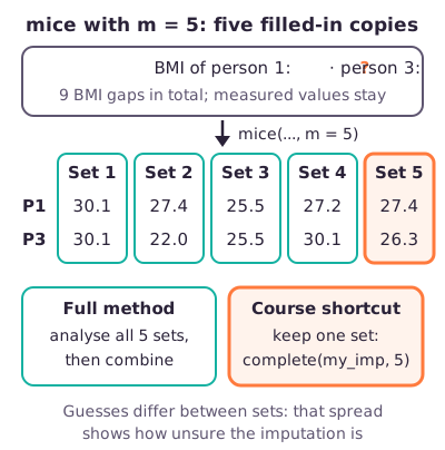
The R package mice (Multivariate Imputation by Chained Equations) fills one incomplete variable at a time with a small prediction model built on the others, then cycles through all variables again for a set number of rounds. It repeats this m times with some randomness, giving m completed datasets whose filled-in values differ slightly: multiple imputation.
The lecture used nhanes, a small dataset that comes with mice: age (complete), bmi (numeric, 9 missing), hyp (hypertension, coded 1 or 2) and chl (cholesterol, numeric).
input_data$hyp <- as.factor(input_data$hyp)
my_imp = mice(input_data, m = 5,
              method = c("", "pmm", "logreg", "pmm"),
              maxit = 20)
my_imp$imp$bmi        # one row per missing BMI, one column per dataset
#       1    2    3    4    5
# 1  30.1 27.4 25.5 27.2 27.4
final_clean = complete(my_imp, 5)
m = 5: five completed datasets.
maxit = 20: 20 rounds through the variables per dataset.
method: one entry per column, in order. "" for age: nothing to impute. "pmm" (predictive mean matching) for numeric bmi and chl: predict the missing value, then copy a real observed value from the person whose prediction is closest. "logreg" (logistic regression, for yes/no outcomes) for hyp.
as.factor(): makes hyp's 1 and 2 two categories, not amounts, so a yes/no method can be used.
complete(my_imp, 5): returns completed dataset number 5. The 5 is an ID, not a quality score.
Figure: Person 1's five guesses range from 25.5 to 30.1. That spread shows how unsure the imputation is.
From the lecture: Why five copies? Run your model on each. If the results differ a lot, the imputation is a big guess; if they are close, it is fairly stable. This is out of scope; picking one completed set is fine for the project.
The full method analyses all m datasets and combines the results.
7. Neural networks versus simple models
The models so far send the inputs through one formula. A neural network sends them through layers of nodes. Each node multiplies its inputs by weights, adds them up, subtracts a threshold, then applies a rule such as "output 1 if above 0, otherwise 0". That on/off step lets stacked layers learn complex, curved patterns.
Worked example: the lecture's surfing node. Inputs: good waves x₁ = 1 (weight 5), empty lineup x₂ = 0 (weight 2), shark-free x₃ = 1 (weight 4); threshold 3. The sum is 1 × 5 + 0 × 2 + 1 × 4 − 3 = 6. Since 6 is above 0, the output is 1: go surfing. An input of 0 contributes nothing, whatever its weight.
From the lecture: Networks learn from labelled examples (supervised learning). A cost function measures how wrong the predictions are, and gradient descent adjusts the weights step by step to lower it. CNNs suit images; RNNs, with feedback loops, suit time series.
Simple model
Neural network
Fits
Simple functions, e.g. a line
Complex functions
Interpretable
Yes
Hardly
Links between inputs
You must handle them
Learned automatically
Bias/variance control
Simple
Needs more attention
Weak point
Fails if data are too complex
Needs much more data
In sport and health you must explain your predictors to a coach or clinician, and a network's hidden nodes are practically impossible to interpret. Networks also need far more data than the course projects have; without it they overfit (learn the noise in the training data instead of the real pattern). So the course uses simple models.
See Lecture 5 for the deep learning versus machine learning trade-off (deep learning extracts features automatically; classical machine learning needs hand-made ones).
8. Risk, odds, RR and OR from a 2×2 table
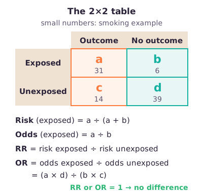
The exposure is what you suspect matters (smoking); the outcome is what you count (heart disease). A 2×2 table crosses them, with cells a and b for the exposed (outcome, no outcome) and c and d for the unexposed.
Absolute risk (AR), a probability: number with the outcome ÷ everyone in the group. Exposed: a ÷ (a + b).
Odds: number with the outcome ÷ number without it. Exposed: a ÷ b.
Relative risk (RR) = risk in the exposed ÷ risk in the unexposed.
Odds ratio (OR) = odds in the exposed ÷ odds in the unexposed = (a × d) ÷ (b × c).
From a probability , : the chance it happens divided by the chance it does not. A probability of 0.75 gives odds of 0.75 ÷ 0.25 = 3.
Figure: Risk divides by the whole row; odds divide by the other cell in the row.
Worked example: 40 of 100 high-load players and 20 of 100 low-load players got injured. Risks: 40 ÷ 100 = 0.40 and 20 ÷ 100 = 0.20, so RR = 2: the high-load group's probability of injury is twice as high. Odds: 40 ÷ 60 = 0.667 and 20 ÷ 80 = 0.25, so OR = 0.667 ÷ 0.25 = 2.67: their odds are 2.67 times as high.
Reading the ratios. For RR and OR alike, 1 means no difference between the groups, above 1 means higher in the exposed group, below 1 lower. Probabilities run from 0 to 1; odds and both ratios from 0 to infinity. An OR is about odds: an OR of 0.5 halves the odds, not the probability, and "14.4 times the odds" is not "14.4 times as likely". A ratio from a table shows an association, not proof of cause.
OR versus RR. For a rare outcome they nearly agree: risks of 8% and 4% give RR = 2 and OR = 2.09. The more common the outcome, the further the OR drifts above the RR (40% versus 20%: RR 2, OR 2.67).
9. Smoking and the pill
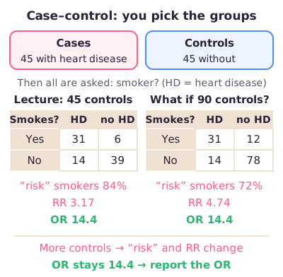
Smoking: why only an OR. The researchers picked 45 patients with heart disease and 45 people without, then asked who smoked.
Heart disease
No heart disease
Smoking
31
6
No smoking
14
39
Worked example: odds of heart disease among smokers are 31 ÷ 6 = 5.17, among non-smokers 14 ÷ 39 = 0.359. OR = 5.17 ÷ 0.359 = 14.4, or (31 × 39) ÷ (6 × 14) = 1209 ÷ 84 = 14.4. Smokers had 14.4 times the odds of heart disease, not 14.4 times the risk.
This is a case–control study: people are picked by outcome (cases with the disease, controls without), then asked about the exposure. The researchers fixed how many had the disease, so a row "risk" such as 31 ÷ 37 = 84% reflects their 45 + 45 choice, not how often smokers fall ill. With 90 controls the "RR" would change but the OR would not: doubling the no-disease column doubles b and d, which cancel in (a × d) ÷ (b × c). Real risks and an RR need a cohort study, which follows exposed and unexposed people forward and counts who develops the outcome.
Figure:Illustration. Doubling the controls moves the "RR" from 3.17 to 4.74; the OR stays 14.4.
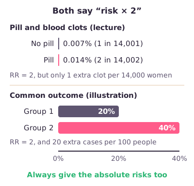
The pill: absolute versus relative risk. What is the risk of a blood clot for women on the contraceptive pill? On the pill, 2 had a clot and 14,000 did not; without it, 1 and 14,000.
Worked example: absolute risk on the pill is 2 ÷ 14,002 = 0.00014 (0.014%); without it, 1 ÷ 14,001 = 0.00007 (0.007%). RR = 0.014 ÷ 0.007 = 2: "the pill doubles the risk". The absolute difference is only 0.007 percentage points (a percentage point is the plain difference between two percentages), about 1 extra clot per 14,000 women. Because clots are rare, the OR is also 2.
So never report a relative risk without the absolute risk. And doubling is a 100% increase, not 200%.
Figure: The same RR of 2 can mean 1 extra case per 14,000 or 20 per 100.
10. Probability, odds and likelihood
Probability: the fraction of times you expect an event over many tries; 0 to 1. Absolute risk is a probability.
Odds: the probability that the event happens ÷ the probability that it does not; 0 to infinity. The odds ratio compares two odds.
Likelihood: how well an assumption or model explains the data you observed. Not the probability of a future event, and not the odds.
Exam traps
Z-scoring keeps the shape; it does not make data normal, whatever the slides suggest. Only log changes the shape.
"When to standardize?" Cheat-sheet answer: roughly normal data, or the algorithm requires it.
Centering alone does not equalize predictors; also divide by the SD.
Log is filed under "normalization" but has no 0–1 range.
KNN table: min–max 0.85, though its code printed 0.77. If a question quotes the table, use the table.
m = number of completed datasets; maxit = number of rounds.
"Odds = 0: no difference" on the slides is wrong: an OR (or RR) of 1 means no difference.
Risk ≠ odds: 20 of 100 is a risk of 0.20 but odds of 0.25.
The slides give R² as an example of likelihood; strictly, R² is variance explained.
The lecturer said probability, odds and likelihood will come up in the exam.
Try the interactive explanation
Open the interactive page: move a height to see its z-score and min–max value, then change event counts to watch AR, RR and OR drift apart.
Worked through the deep dive?Tick it off. Come back to any section whenever you need it.
3Step 3 of 35–8 min
Practice questions
3 exam-style questions. Exam-style open questions: short, with the points shown like on the real exam. Write your answer in the box, then check it against the model answer and the marking guide.
Question 1 — Z-score and min–max (2 points)
For a KNN model, countermovement jump height is scaled with values from the training set: mean 50 cm, SD 10 cm, minimum 20 cm, maximum 80 cm. A new athlete jumps 65 cm. Calculate and show your working: 1) the athlete's z-score (1 point) 2) the athlete's min–max value (1 point)
Show answer and rationale
1) z = (65 − 50) ÷ 10 = 1.5: the athlete is 1.5 SD above the training mean.
2) min–max = (65 − 20) ÷ (80 − 20) = 45 ÷ 60 = 0.75: the athlete is 75% of the way from the training minimum to the maximum.
How the points are earned
1 pt z = (65 − 50) / 10 = 1.5
1 pt min–max = (65 − 20) / (80 − 20) = 0.75
How did your answer compare?
Question 2 — Scaling before KNN (3 points)
A KNN model classifies athletes as sprinters or endurance athletes from height (in metres) and body mass (in kg), without any scaling. State and motivate briefly: 1) Why should you rescale these features before fitting KNN? (1 point) 2) Explain the difference between z-score standardization and min–max normalization, and say whether either one makes a skewed feature normally distributed. (2 points)
Show answer and rationale
1) KNN classifies by distances. Body mass differs by tens of kg and height by tenths of a metre, so body mass dominates every distance and height hardly counts. Rescaling puts both on comparable ranges, which can change which neighbours are chosen and so the prediction.
2) Z-score: (value − mean) ÷ SD, giving mean 0 and SD 1, with no fixed range. Min–max: (value − minimum) ÷ (maximum − minimum), giving values from 0 to 1. Neither makes a skewed feature normal: both only shift and rescale, so the shape of the distribution stays the same (a log transformation would change the shape).
How the points are earned
1 pt KNN uses distances; without scaling the feature with the largest numbers (body mass) dominates
1 pt Correct description of both: z-score gives mean 0 and SD 1; min–max gives range 0–1
1 pt Neither makes the data normal: both keep the shape of the distribution
How did your answer compare?
Question 3 — Risk, odds and reporting (3 points)
In one season, 50 of 100 players with a high training load and 20 of 100 players with a low training load got injured. State and motivate briefly: 1) Calculate the relative risk (RR) and the odds ratio (OR) of injury for high versus low load. (2 points) 2) Write one sentence that reports this result the way the lecture recommends. (1 point)
Odds: 50 ÷ 50 = 1 and 20 ÷ 80 = 0.25, so OR = 1 ÷ 0.25 = 4. The OR is larger than the RR because injury is common here.
2) 'Injury occurred in 50% of high-load players versus 20% of low-load players: 2.5 times the risk, or 30 percentage points more.' Always give the absolute risks with the relative risk; the table shows an association, not proof of cause.
How the points are earned
1 pt RR = 0.50 / 0.20 = 2.5
1 pt OR = (50/50) / (20/80) = 4
1 pt Sentence gives the absolute risks (50% vs 20%, or 30 percentage points) together with the relative measure