Lecture 8 is a guest lecture on data in environmental health. It follows one study from question to result: is long-term exposure to nitrogen dioxide (NO₂), a traffic gas, linked to death among Dutch adults?
The ideas to keep
Blur the explanations and test yourself.
Hazard, exposure, risk. A hazard is something that can harm (NO₂, a shark in the sea). Exposure is how much of it you meet and for how long. Risk is the chance of actual harm and needs both. Studies follow four steps in order: identify the hazard, characterize it (harm as a function of dose), assess exposure, characterize risk.
A precise question. Fixing area, population, exposure, outcome and time frame decides which data you need. Here: adults over 30 in the Netherlands, NO₂, death from any cause, a 10-year average.
Home address as a proxy. Nobody can measure what thousands of people breathe everywhere, so NO₂ at each home address is the stand-in. It must be address-specific because NO₂ drops sharply within metres of a busy road.
Land-use regression. NO₂ was measured at only 69 stations. Land-use regression learns how measured NO₂ depends on nearby roads and green space, then predicts it at every home. It is checked on stations left out of the fit. This exposure model feeds a separate health model (a Cox survival model), so its errors carry over.
Health data have limits. National registries are big, cheap and consistent but shaped by paperwork: more deaths are registered on Mondays because of registration practice, not biology. Questionnaires depend on wording. Biomarkers (disease signs measured in the body) are early but costly and invasive.
Confounding. A third factor that drives both exposure and outcome, such as income or smoking, can fake or distort a link, so a plain correlation is not enough. The model adjusts for confounders, but only the measured ones.
Reading HR = 1.04. A hazard ratio compares death rates for a stated step in exposure. HR 1.04 means a 4% higher death rate per step: not 104%, and not 4 percentage points. It is significant, since its 95% confidence interval (1.03–1.04) excludes 1. Its public-health weight depends on how many people are exposed and how much, and it shows association, not cause.
What to be able to do
Label hazard, exposure and risk in a scenario; order the four risk-assessment steps.
Choose exposure data for a question, with a pro and a con for campaigns, routine networks and satellites.
Give the four land-use regression steps, its outcome and predictors, and its validation; contrast it with a physics-based model.
Classify a model as parametric, semi-parametric (Cox) or non-parametric.
Explain why a correlation fails here, using a confounder.
Tell RR, OR and HR apart (RR and OR are computed as in Lecture 7).
Read Cox output in R and interpret an HR with its increment, confidence interval and limits.
Got the big picture?Mark the overview done to fill this lecture's ring.
2Step 2 of 312–18 min
Detailed notes
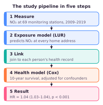
This lecture follows one environmental-health study from question to result: is long-term exposure to traffic air pollution (NO₂) linked to death among Dutch adults?
Nitrogen dioxide (NO₂) is a gas from burning fuel, mostly traffic. The study joined two kinds of data per person:
Exposure. NO₂ was measured at only 69 monitoring stations. A land-use regression model learned how NO₂ depends on the roads and land use around each station, then predicted it at every home address.
Health. National person-level records from Statistics Netherlands (CBS) gave who died and when, plus age, sex, smoking, income and more.
Linking. Each person got the predicted 10-year average NO₂ at their address.
Modelling. A Cox survival model compared death rates across NO₂ levels, adjusting for other differences between people.
Result. A hazard ratio of 1.04, and three questions: is it significant, is it big, is it causal?
Figure: Steps 1–2 estimate exposure, step 3 joins the data, steps 4–5 estimate the health association. Every step can add error, and a big dataset does not repair bad data.
2. Environmental health: hazard, exposure, risk
Health and environment. The WHO's 1948 definition calls health complete physical, mental and social well-being, not just the absence of disease. Critics call that unrealistic, since hardly anyone is completely well for long; a newer definition sees health as the ability to adapt and self-manage. The environment covers both the natural environment (air, green and blue spaces) and the built environment (houses, roads, neighbourhood design).
Environmental health is the part of public health, the health of whole populations, that covers physical, chemical and biological factors outside a person, plus behaviour linked to them (such as cycling more because a town is built for it). It excludes behaviour unrelated to the environment, the social and cultural environment, and genetics. Typical problems: heat, air pollution, noise, pesticides and microplastics.
Hazard, exposure and risk. A hazard is something with the potential to harm. Exposure is how much of it you meet and for how long. Risk is the chance it actually harms you, and it needs both. A shark is a hazard: dangerous, but you only face a risk if you swim near it, and the risk grows with how long and how close. In the study, NO₂ is the hazard, the 10-year average at home is the exposure, and the chance of dying earlier is the risk. Exposure is not dose, the amount that actually enters the body.
The risk assessment paradigm is the standard four-step route, in this order:
Step
Question
NO₂ example
1. Hazard identification
Can the agent harm an exposed population?
Does NO₂ harm health at all?
2. Hazard characterization
How do the probability and severity of harm depend on the dose?
How much harm per µg/m³ (dose–response)?
3. Exposure assessment
What levels, types and durations of exposure, in which population?
Who breathes how much, for how long?
4. Risk characterization
What are the consequences at current levels, and what would less exposure gain?
How many deaths now, and how many fewer with cleaner air?
Four approaches split the paradigm between them:
Approach
Studies
Serves
Toxicology
how, when and why hazards are toxic
the hazard (steps 1–2)
Physiology
how the body responds to environmental factors
the hazard (steps 1–2)
One Health
how people, animals, plants and ecosystems interact
exposure and risk (steps 3–4)
Environmental epidemiology
how disease is spread in a population and which environmental factors drive it
exposure and risk (steps 3–4)
The study uses environmental epidemiology.
3. The research question
Before collecting data, fix five things. Each choice decides which data you need.
Factor
Choice in the study
Area
the Netherlands
Population
adults over 30
Exposure
NO₂
Outcome
all-cause mortality (death from any cause)
Time frame
long-term (10 years)
The question became: what is the risk of mortality related to long-term exposure to ambient (outdoor) NO₂ in adults in the Netherlands? The population is a cohort, a fixed group followed over time: 33,475 adults followed from 2009 to 2019. A short-term question, such as asthma attacks the day after high pollution, would need daily or hourly data instead.
4. Exposure data: the home-address proxy and its sources
What you really breathe changes as you move between micro-environments (home, street, office, train, gym). Measuring that for thousands of people over 10 years is not feasible. So the study uses the average NO₂ at each person's home address as a proxy, a stand-in measure. It assumes people spend most (not all) of their time at home.
The value must be address-specific because NO₂ varies strongly over short distances: very high next to a busy road, much lower a few streets away. One city or national average would give everyone nearly the same value and leave no differences to compare. The limitation: the proxy misses exposure at work, while commuting and before a house move, so the study estimates the effect of home-address NO₂, not of what people actually inhaled.
Measurements come from two kinds of source. Spatial resolution, how small an area one value describes, matters when exposure changes within metres.
Source
Pros
Cons
Designed campaign: your own fixed sites or mobile monitors
you choose pollutants and locations
high cost; cannot cover large populations; quality can be poor
Routine network, surface: permanent government stations
low cost; long periods; continuous; several pollutants at once
your pollutant may not be measured; no or too few stations in your area; quality can be poor
Routine network, remote sensing (satellites)
free; wide coverage; long time series
coarse resolution (about 1–25 km per value)
Use a routine network for long-term, large-population studies, and a designed campaign when you need a specific pollutant or place.
5. Exposure models: deterministic versus land-use regression
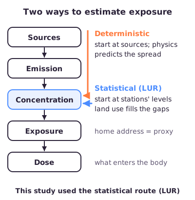
If you live between two stations, what level do you get? A model must interpolate, estimating values between measured points. Two model families enter the chain from sources to dose at different points.
Figure: Deterministic models start at the sources; statistical models start from measured concentrations.
Deterministic
Statistical
Also called
dispersion or chemical transport model
land-use regression (LUR)
Starts from
pollution sources and their emissions
concentrations measured at stations
Predicts by
physical and chemical laws of how pollutants spread
a learned link between measured levels and surrounding land use
The study used LUR, in four steps:
Measure concentrations at a limited number of sites: here 69 stations over 10 years.
Choose predictors about traffic and land use, such as road length, residential, industrial and green areas, and population. Each is counted within buffers, circles of a chosen radius (50 m to 10 km) around the point.
Fit a regression that explains the differences in NO₂ between stations, usually multiple linear regression or machine learning.
Apply it to unmeasured locations, such as every participant's home address.
The regression in step 3 has this form:
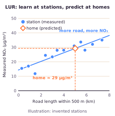
In words: NO₂ at a station () equals a constant plus, for each land-use feature , its coefficient times how much of that feature surrounds the station. Stations with more road nearby have higher NO₂, so roads get a positive coefficient; green space gets a negative one.
Figure: LUR with one predictor. Dots are stations, the line is the learned rule, the diamond is a home with no measurement.
Worked example: (Illustration: invented stations, as in the figure.) The fitted rule is NO₂ ≈ 14.3 + 2.98 × (km of road within 500 m). Here 14.3 µg/m³ is the background level with no road nearby, and 2.98 is the coefficient: each extra km of road adds about 3 µg/m³. A home with 5 km of road nearby gets 14.3 + 2.98 × 5 ≈ 29 µg/m³. A real LUR does this with many predictors at once.
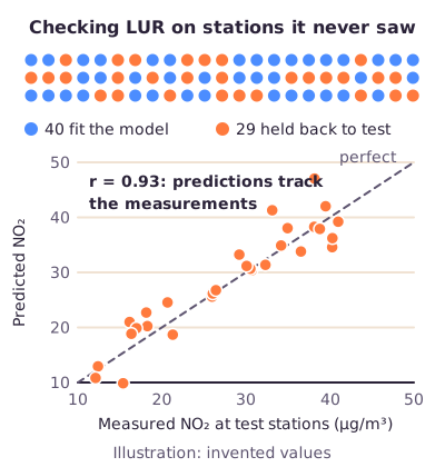
Challenges: the quality of the monitoring data (bad input makes the model meaningless, so check it first), choosing the right model, model uncertainty, and validation. Validation is usually a hold-out check: fit the model on part of the stations (for example 40 of the 69), predict the stations left out, and compare the predictions with their measurements.
Figure: A hold-out check (invented values). Points near the dashed line mean good predictions at stations the model never saw.
Good test predictions are reassuring, not proof: at places never measured you still assume the model works. Judging the model only on the stations it learned from rewards overfitting, fitting those 69 stations so closely that it predicts badly elsewhere.
Keep the two models apart. LUR is the exposure model: it predicts NO₂ from land use. The Cox model (Section 11) is the health model: it links that NO₂ to death. Errors in the first flow into the second.
6. Health data
A 2020 review by Galetsi and colleagues groups big health data into four categories:
Category
Contains
Clinical
clinical endpoints, such as new cases of disease and deaths
Real-time patient
wearable-sensor data, such as heart rate and steps
Administrative
costs and reimbursements of medical expenses
Pharmaceutical
toxicological data (effects of drugs) and medicine use
From the lecture: Clinical data are often too sensitive to access, so administrative data can stand in: you may not see the diagnosis, but you can see who paid for certain therapies.
large numbers, often the whole country; sometimes the only option for very rare diseases; cheap; consistent
quality of information; completeness; depends on administrative factors; privacy regulations
Questionnaires: symptoms, quality of life, medication, lifestyle
large surveys; cheap
wording; hard to compare between questionnaires; mode of administration (interview or written)
Physiological measurements: biomarkers, signs of disease measured in the body
earlier in the chain from exposure to disease; possibly less bias than clinical outcomes
can be invasive; expensive and slow; instrument and observer effects
From the lecture: More deaths are registered on Mondays than on Sundays. That is not biology: registration practice and medical shifts push weekend deaths into Monday's records. This is what "depends on administrative factors" means.
The study's outcome is death across a whole country, so it used a registry: CBS microdata, person-level records on everyone registered in the Netherlands (deaths, illness, income, housing and more), available only to approved researchers and not free. The challenges are choosing an endpoint that fits the exposure, privacy rules, completeness (enough events to analyse), and processing, usually the most time-consuming step.
7. Linking, processing and privacy
A registry gives a date of death, not an outcome column. You derive it: died between 2009 and 2019 = 1, otherwise 0. The final table has one row per person: ID, age at the start and end of follow-up, sex, smoking and other confounders coded as numbers, home coordinates, the predicted 10-year NO₂, and the 0/1 outcome.
Errors creep in at every join: an unrepresentative station, an outdated address, exposure assigned to the wrong period, a missing death record, or sources that define the endpoint differently. A large sample removes none of them. Over 10 years people move, so long-term exposure should ideally follow each person's residential history, every address with its dates.
From the lecture: Removing names does not make person-level data anonymous: address, age and sex can re-identify someone. CBS data are therefore used only after an approved proposal, inside a secure remote environment, with only the approved variables, and results are checked before export (a minimum number of people per reported cell).
8. Analysis plan: describe, then model
The analysis has two goals: a quantitative estimate of risk with its uncertainty, and a correct interpretation of the model output. It runs in two steps.
Descriptive analysis summarises who is in the data and what the exposure and outcome look like, with tables and plots and no model. Here: 33,475 people, three-quarters women, mean age 49.7 at the start, and residential NO₂ of 25.41 ± 4.80 µg/m³ (mean ± standard deviation), range 11.23–44.11. This catches odd values and missing data early and shows whom the results apply to.
Association analysis then estimates how strongly exposure and outcome go together, with its uncertainty: here, the Cox model's hazard ratio. Models differ in how much they fix the functional form, the shape of the exposure–outcome relationship:
Family
Shape
Examples
Parametric
fixed in advance: linear or polynomial (such as a parabola)
simple linear regression, conditional logistic regression
Semi-parametric
partly fixed, partly free
local models, generalized additive models (sums of smooth curves), Cox model
Non-parametric
inferred from the data
random forest, decision trees, boosting
Every model has assumptions, such as normality, independence or linearity, and cannot be applied blindly; flexible does not mean assumption-free. To choose, look at what others used for similar questions and at your own data.
9. Why not a correlation? Confounding
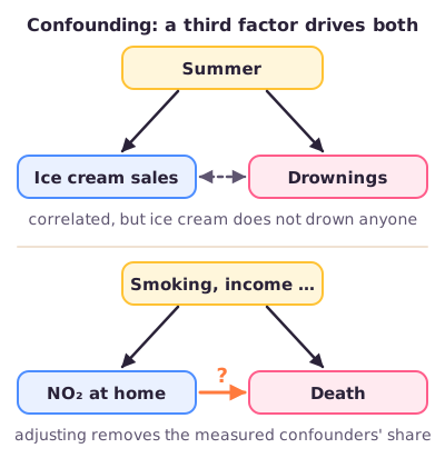
A correlation coefficient between NO₂ and death is simple, but not a useful measure of association here, because of confounding. A confounder is a third factor that affects both the exposure and the outcome, so it can create a link that is not there or distort a real one. The lecture's example: ice cream sales and drownings rise together because both go up in summer, not because ice cream drowns people.
Figure: The same structure in both cases. The orange arrow is what we want to estimate.
In the study, where you live is linked to income, and income to smoking, diet and health. If poorer neighbourhoods are both busier with traffic and less healthy for other reasons, NO₂ would look deadlier than it is. So the Cox model adjusts for confounders: it includes them, so NO₂ is compared among people who are otherwise alike. Here these included smoking, BMI, education, diet and neighbourhood income. Adjustment only removes confounders that were measured, and only as well as they were measured.
10. RR, OR and HR
All three are measures of association: they compare how often the outcome happens in a more exposed group versus a less exposed one. For all three, 1 means no difference, above 1 means more events with more exposure, and below 1 fewer. They are different numbers and not interchangeable.
The relative risk (RR) divides the risk (the share who get the outcome) in the exposed group by that in the unexposed group. The odds ratio (OR) divides their odds (events ÷ non-events), and is close to the RR only when the outcome is rare. See Lecture 7 for how to compute RR and OR.
The hazard ratio (HR) comes from a Cox model. A hazard here is the instantaneous risk: how fast the event is happening right now among people who have not had it yet. It is a rate, such as deaths per 1,000 person-years (everyone's follow-up time added up). The HR compares two hazards, either between two groups or for a fixed increment in exposure, such as 10 µg/m³ more NO₂. It compares rates at each moment, not the chance of having died by the end.
11. The Cox model and its R output
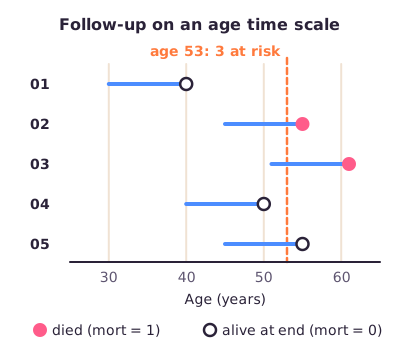
Survival analysis (time-to-event analysis) studies how long until an event happens, not only whether it happens. The Cox proportional hazards model is one of the most used models for long-term survival studies. Here time is measured as age: each person enters at their age at the start (age_b) and leaves at their age at the end (age_end), either at death (mort = 1) or at the end of follow-up (mort = 0). At any age, the people at risk are those still followed and alive.
Figure: Five people from the lecture's example table, each line from age at start to age at end; a filled dot means died. At age 53, persons 02, 03 and 05 are at risk, and the hazard at 53 is about deaths among exactly these people.
In words: a person's hazard at time is the baseline hazard at that time, multiplied by e raised to a weighted sum of their exposure (NO₂) and confounders , with coefficients .
, the baseline hazard, is the hazard of someone whose variables are all 0. It changes with age, and the model leaves its shape free. That free part makes Cox semi-parametric; the exp( ) part has a fixed form.
One unit more NO₂ multiplies the hazard by , so HR = e^b: the coefficient is the log of the hazard ratio.
Proportional hazards: the ratio between two people's hazards is the same at every age, even though both rates rise with age.
The model formula in R (shortened), passed to a Cox function such as coxph():
coef is the log hazard ratio (negative means a lower hazard); exp(coef) is the hazard ratio itself.
se(coef): the standard error, how uncertain the coefficient is.
z = coef ÷ SE. Beyond about ±2 means significant at the 5% level.
Pr(>|z|): the p-value, the probability of an association at least this strong if there were truly none; *** means below 0.001.
Worked example: reading the rows.
Smoking: exp(0.32) = 1.377, the printed HR: about a 38% higher hazard.
Employed: exp(−0.18) = 0.835, an HR below 1: a 16.5% lower hazard. A negative coefficient always gives an HR below 1; the HR itself is never negative.
NO₂: z = 0.00392 ÷ 0.000246 = 15.93, far beyond 2, so p < 2 × 10⁻¹⁶.
12. Reading HR = 1.04
The headline result: HR = 1.04 (95% CI 1.03–1.04), p < 0.001, adjusted for the confounders in Section 9. One correct sentence: after adjustment, each increment higher in long-term home NO₂ was associated with a 4% higher hazard of death.
The increment is the exposure step the HR refers to, and an HR means nothing without it. The lecturer's example increment was 10 µg/m³, which is also the step the printed coefficient fits.
Worked example: what HR 1.04 per 10 µg/m³ means. (Illustration: the baseline rate is invented.)
Two people, alike in every adjusted factor: Anna lives at 20 µg/m³ NO₂ and Ben at 30 µg/m³. Ben is one increment (10 µg/m³) higher.
Anna's hazard at age 60: suppose 10 deaths per 1,000 person-years (about 10 deaths a year among 1,000 people like her).
Ben's hazard: 10 × 1.04 = 10.4 per 1,000 person-years. That is "4% higher hazard": his rate is Anna's multiplied by 1.04.
In absolute terms that is 0.4 extra deaths per 1,000 person-years. It is not 4 percentage points more deaths (that would add 40 per 1,000), and not "104% risk" (that would roughly double the rate).
Proportional hazards: at 70, if Anna's hazard is 25 per 1,000, Ben's is 26. The ratio stays 1.04 as both rates rise.
Two increments (20 µg/m³ apart): 1.04 × 1.04 = 1.08, about 8% higher.
What it does not say: that NO₂ caused Ben's extra 0.4 deaths. It is an association in observational data, adjusted only for measured confounders (Section 13).
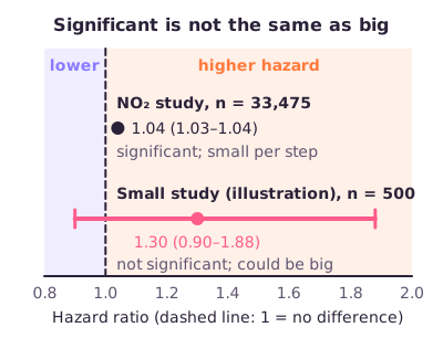
Significant? Yes. The 95% confidence interval (CI), the range of HR values compatible with the data, runs from 1.03 to 1.04 and excludes 1, and p < 0.001.
Substantial? Per person, 4% per step is modest. But an HR is not a measure of health burden, the total harm in a population, which depends on how many people are exposed, to which levels, and on the baseline death rate. With the rates above, 0.4 extra deaths per 1,000 person-years across one million exposed people is about 400 extra deaths a year. And a big study makes even a small HR significant, because its interval is narrow.
Figure: Significance is about how sure we are that the HR is not 1; size is about how far it is from 1. The small study is invented.
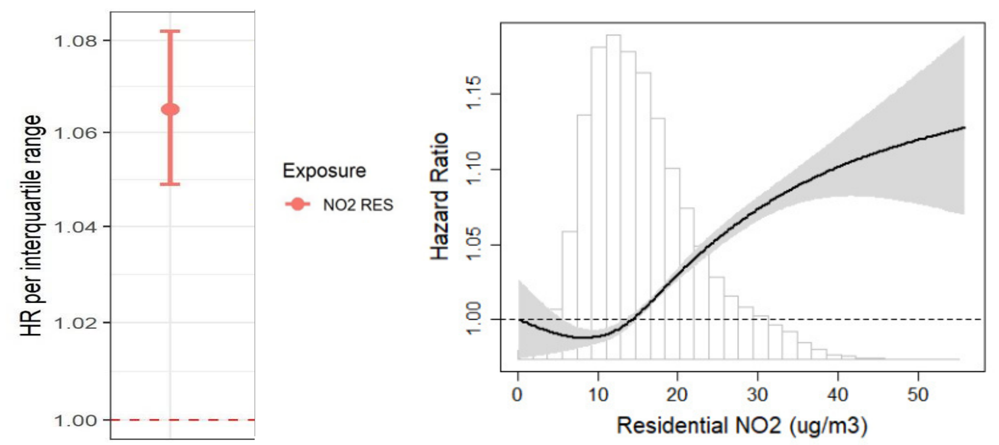
The exposure–response curve shows the HR across the whole range of NO₂.
Figure: The study's results. Left: the HR per interquartile range of NO₂. Right: the hazard ratio across residential NO₂, with its uncertainty band (grey) and a histogram of how many people live at each level.
Left: the HR per interquartile range (IQR), the spread of the middle half of exposures (75th minus 25th percentile): about 1.065, CI about 1.05–1.08. Same data, different increment, different number.
Right: a spline, a flexible curve built from short joined pieces so its shape can change along the x-axis. The HR stays near 1 up to about 15 µg/m³ (dipping slightly below it), then rises to about 1.10 at 40 and 1.13 at 55. The band widens at high levels because few people live there.
Reading: risk rises with concentration, but not in a straight line, so one HR per step only summarises the curve.
13. Association, not causation; the case as a whole
This is an observational study: researchers recorded where people lived and whether they died, and nobody was assigned to breathe more NO₂. So the result shows that higher NO₂ is associated with a higher death rate after adjustment, not that NO₂ caused those deaths. Reasons for caution:
the exposure is a proxy: home-address NO₂, not what people breathed;
the data are heavily modelled: predicted by LUR, then linked, with error added at each step;
residual confounding: only measured confounders were adjusted for;
results can change with the population's size and make-up.
Confidence comes from replication (similar results in other populations, such as Belgium), consistent results within subgroups (such as among low-income people only, which makes confounding by income less likely), and evidence from other approaches, such as toxicology showing that NO₂ is harmful.
From the lecture: The course lecturer asked students to spot the data science lifecycle from Lecture 1 here: the problem (five factors), acquisition (stations, CBS microdata), preparation (0/1 outcome, linking), exploration (descriptive tables), features (land-use buffers), modelling (LUR, Cox), visualization (maps, HR plots) and communication (conclusions with limitations).
Overall, exposure and health data must be checked and correctly processed, and every choice depends on the research question and aim, resources, time, and data availability and quality.
Exam traps
HR increment: the lecture's conclusion says HR 1.04 is "per 1-unit increase", but the coefficient gives 1.04 only per 10 µg/m³ (per unit, ), and the plot shows 1.065 per IQR; use the increment the question states.
HR 1.04 = 4% higher hazard. Not "104% risk", not 4 percentage points, not "NO₂ causes 4% of deaths".
An HR is never negative: a negative coefficient means HR < 1 (the speaker said "negative hazard ratio").
Surv(...) defines the outcome (follow-up and death), not the baseline hazard (as the speaker called it).
"Hazard" in hazard–exposure–risk is the agent (NO₂); in survival analysis it is a rate.
The step labelled "predictive analyses" estimates an association, not individual forecasts.
Significant (CI excludes 1) is not substantial (needs numbers exposed, levels, baseline rate).
LUR's outcome is NO₂ at stations; mortality is the Cox model's outcome.
Monday deaths are an administrative artefact: not real, not confounding.
Try the interactive explanation
Open the interactive page and drag the exposure step to see how HR 1.04 compounds; it uses the per-1-unit reading (see Exam traps).
Worked through the deep dive?Tick it off. Come back to any section whenever you need it.
3Step 3 of 35–8 min
Practice questions
2 exam-style questions. Exam-style open questions: short, with the points shown like on the real exam. Write your answer in the box, then check it against the model answer and the marking guide.
Question 1 — Exposure data for a city study (3 points)
You want to study whether long-term exposure to traffic-related NO₂ is associated with hospital admissions in adults living in Amsterdam. State and motivate briefly: 1) Why is one city-wide annual average NO₂ value not a good exposure measure, and what would you use instead? (2 points) 2) Name one confounder you would adjust for and explain why it is a confounder. (1 point)
Show answer and rationale
1) NO₂ changes strongly over short distances: very high next to busy roads, much lower a few streets away. One city-wide value gives every person the same exposure, so there is no difference between people to relate to admissions. Instead, give each person a long-term NO₂ estimate at their home address, for example predicted with a land-use regression (LUR) model (ideally following their address history if they move).
2) For example income: people with a lower income more often live near busy roads and also have poorer health for other reasons, so income affects both the exposure and the outcome and can distort the link. Smoking or age are also acceptable with a similar reason.
How the points are earned
1 pt NO₂ varies strongly over short distances, so one city value gives everyone the same exposure (no contrast)
1 pt Use a long-term estimate per home address, e.g. from land-use regression (LUR)
1 pt Valid confounder (e.g. income, smoking, age) that is linked to both the exposure and the outcome
How did your answer compare?
Question 2 — Interpreting a hazard ratio (3 points)
An observational cohort study reports the result below for death from any cause. State and motivate briefly: 1) Interpret this hazard ratio in one sentence. (1 point) 2) Is the association statistically significant? (1 point) 3) Name one conclusion you cannot draw from this result, and why. (1 point)
Adjusted Cox model
NO2 (per 10 µg/m³ higher): HR = 1.06 (95% CI 1.02–1.10)
Show answer and rationale
1) After adjustment for confounders, people with 10 µg/m³ higher NO₂ exposure had a 6% higher hazard (instantaneous death rate).
2) Yes: the 95% CI (1.02–1.10) does not include 1.
3) One of: you cannot conclude that NO₂ causes the deaths, because the study is observational and unmeasured confounders may remain; you cannot read it as 6 percentage points more deaths, because an HR is a relative measure and the baseline death rate is not given.